COMET is used to check and design the most common types of joints of steel bar structures used in civil and industrial engineering. The application enables to perform checks for compliance with requirements of one of the following design codes
and to design a steel structural joint based on a particular prototype.
Unlike invention, the prototype-based engineering involves using available designs. This approach is implemented in COMET, and is based on selecting from a set of parameterized standard structural designs of joints (prototypes). Parameters of a prototype depend on the specified design conditions (material, internal forces etc.), and cannot be determined independently because certain relationships usually exist between them.
COMET uses the above approach and thus enables the engineer to improve the efficiency of his work by providing him with a wide range of prototypes. In this way the highly qualified personnel does not have to do the routine technical work of checking and correcting a multitude of parameters to comply with building codes and design specifications.
Once a design is selected for the joint, the application enables to determine all its parameters, which must comply with the standard requirements, a number of structural constraints, and the assortment of steel members. Both the standard requirements and structural constraints provided in the codes are obligatory, and their violation is not allowed. However, there are also certain design constraints violating which would cause only a warning, and the application can generate a solution with such violations.
The initial data for computer-aided design of steel structural joints include a configuration or type of the joint, type and sizes of cross-sections of bearing members connected in this joint, and internal forces acting in these members for an arbitrary number of design combinations of loadings.
On the Design stage (after clicking the respective button) the software performs the selection of a rational design of the joint which satisfies all the requirements and a set of structural and assortment limitations. The user can either accept the suggested solution or modify it according to his preferences, in order to take into account:
On the Calculate stage (after clicking the respective button) a check of the design of the joint is performed and a drawing (a sketch of the joint design with all its parameters close to the MS (metal structures) stage) is generated. In order to be able to modify the design thus generated, or to alter the format of representation of drawings (e.g., dimensioning, legends etc.), the graphical results can be exported as a DXF (AutoCAD) file.
All design modes of the application (except for the Beam-To-Column Joints mode) assume that all members connected in the joint and all auxiliary members of the joint (gussets, stiffeners, angle cleats etc.) are made of the same steel.
Check and design of joints are usually performed for the action of several load cases or their combinations, which can be specified by the user. It should be noted that the sequence of specification of the load combinations can in some cases affect the result of the design.
According to their structure, prerequisites, checks, structural limitations and recommendations SNiP II-23-81*, ShNK 2.03.05-13, SP 53-102-2004, SP 16.13330, DBN B.2.6-163:2010 and DBN B.2.6-198:2014 are quite close documents. Since the set of problems which can be solved in COMET is the same for these documents, all the general references to SNiP ІІ-23-81* found in the text should be treated as similar references to ShNK 2.03.05-13, SP 53-102-2004, SP 16.13330, DBN B.2.6-163:2010 or DBN B.2.6-198:2014.
Design codes are developed as a system of checks of the known design, i.e. they solve the problem of structural assessment rather than the problem of its synthesis. Comet enables to solve both these problems — assessment task and selection task. However, the latter problem (selection) is solved in a limited formulation as a purposeful search through the list of possible designs.
The described approach to the selection (synthesis) of the cross-section leads to designs that for one reason or another (design considerations, unification, etc.) may not satisfy the designer. He can adjust the design proposed by the program and perform its verification in the check mode.
Standard requirements (conditions of strength, general and local stability, limit slenderness, etc.) to a certain design section of a structure can be written in the form of a certain system of inequalities, each of which depends functionally on the values of internal forces \( \vec{{S}} = \{ S_{1}, S_{2}, ... , S_{n} \} \) that can arise in the considered section from the action of the design combinations of loadings:
\[ {\rm {\bf \Phi }}\left( {\vec{{S}},\vec{{R}}} \right)\le 1 ;\]
or
\[ \left\{ {{\begin{array}{*{20}c} {f_{1} \left( {\vec{{S}},\vec{{R}}} \right)\le 1;} \\ {f_{2} \left( {\vec{{S}},\vec{{R}}} \right)\le 1;} \\ {...} \\ {f_{j} \left( {\vec{{S}},\vec{{R}}} \right)\le 1;} \\ {...} \\ {f_{m} \left( {\vec{{S}},\vec{{R}}} \right)\le 1;} \\ \end{array} }} \right. ,\]
where n is the total number of possible internal forces in the section; m is the number of inequalities that describe the standard requirements; fi is a function of principal variables that implements j-th check; R are generalized resistances.
Based on the values of functions \( K_{j} =f_{j} \left( {\vec{{S}},\vec{{R}}} \right) \), we can introduce the concept of a utilization factor of restrictions, and thus represent the analysis criterion as:
\[ K_{\max } =\max \left\{ {K_{j} \quad \vert \quad j=1,...,m} \right\}\le 1 , \]
where \(К_j\) is the left-hand side of the design inequality \( f_{j} \left( {\vec{{S}},\vec{{R}}} \right)\le 1 \),
where required analyses are included. The value of Кj itself will define a reserve of strength, stability, or another regulated quality parameter available for a particular element (joint, connection, cross-section etc.). If the requirement of the design code is met excessively, then Кj is equal to the relative value of exhaustion of the design requirement (for example, Кj = 0,7 corresponds to the reserve of 30%). If the design requirements are not met, the value of Кj > 1 indicates a violation of a requirement, i.e. it describes a degree of overloading.
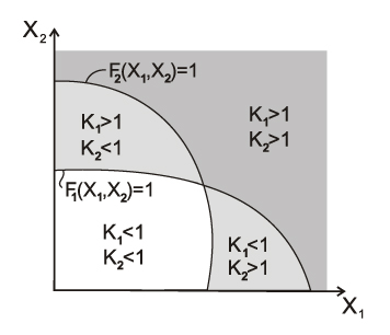
Each standard requirement \( K_{\max } =\max \left\{ {K_{j} \quad \vert \quad j=1,...,m} \right\}\le 1 \) defines a certain area Ωj in the n-dimensional space of internal forces, and the intersection of all areas Ωj forms the load-bearing capacity area of the section Ω in terms of the considered codes (Fig. 1). The maximum utilization factor of restrictions for each point of the load-bearing capacity area of the section is \( K_{\max } =\max \left\{ {K_{j} \quad \vert \quad j=1,...,m} \right\}\le 1 \).
Figure 1. Formation of the load-bearing capacity area in the two-dimensional space of internal forces
Regulatory restrictions are usually written as follows:
\[ \varphi_{j} \left( {\vec{{S}}} \right)\le \psi_{j} \left( {\vec{{R}}} \right), (j = 1, …,m), \]
where φj, ψj – functions of the main variables which implement the j-th check.
However, not all these requirements can or need to be rewritten in the form:
\[ f_{j} \left( {\vec{{S}},\vec{{R}}} \right)\le 1, (j = 1,…, m), \text {where} \] \[ f_{j} \left( {\vec{{S}},\vec{{R}}} \right)=\frac{\varphi_{j} (\vec{{S}})}{\psi_{j} (\vec{{R}})}, \]
i.e. in the form of the ratio of the left-hand side of the standard inequality to its right-hand side.
To illustrate this let’s consider formula (8.78) of SP 63.13330.2012 as an example:
\[ T\le T_{0} \sqrt {1-\left( {\frac{M}{M_{0} }} \right)^{2}}. \]
If the following ratio was calculated as the value of the utilization factor of this standard check:
\[ \frac{T}{T_{0} \sqrt {1-\left( {\frac{M}{M_{0} }} \right)^{2}} }\le 1, \]
then in the design situation when M < M0, we would obtain a root from a negative number in the denominator, and would not be able to obtain a quantitative estimate of the excess of the bearing capacity, which is avoided by transforming the formula (8.78) as follows:
\[ \left( {\frac{T}{T_{0} }} \right)^{2}+\left( {\frac{M}{M_{0} }} \right)^{2}\le 1. \]
The numerical value of the factor (the value of the utilization factor of restriction) is a measure of how fully the bearing capacity of the structural member is used (or how much it is exceeded), and as a result it allows the designer to make a correct decision about the type of the necessary design modification and only! For example, it hardly makes sense to select another steel grade with a greater design strength in the case when the stability check turned out to be critical.
It should be specially emphasized that there may be no direct proportionality between the value of the factor and the values of the forces appearing in the standard check, as there may be no direct proportionality between the value of the factor and the values of the geometric properties of the cross-sections of the structural elements. This is due to the non-linearity of the standard checks, in particular, the non-linearity of the function of the buckling coefficient, etc.
All values of the Кj factors obtained by analysis are given in the Factors Diagram dialog box or in a full report document. The respective dialog boxes display the value of Кmax – the maximal (i.e., the most dangerous) among the detected Кj values and indicate the type of check (e.g., strength, stability) in which this maximum took place.
The data given in the diagram of factors enable the designer to make a correct decision on the type of necessary structural modifications. For instance, it hardly makes sense to increase the design strength of steel if the stability check turned out to be the critical one.
Sections of bar elements, where six internal forces (longitudinal force, bending moments, transverse forces, and torque) can appear under the load, have a load-bearing capacity area in the form of a six-dimensional geometric object which is very difficult to analyze. The best way to display the load-bearing capacity area of sections is by performing its orthogonal projection onto a certain plane (pair) of internal forces. The generation of a two-dimensional projection of the load-bearing capacity area of a section is performed according to the algorithm given below.
The user selects a pair of internal forces (for example, a pair “longitudinal force N – bending moment My”), in the coordinate system of which an orthogonal projection of the load-bearing area will be generated. The remaining internal forces in the section (Mz, Qy, Qz, Mx) are fixed at a certain level (they are specified by the user or take zero values). At a certain fixed value of the ratio e = My/N, the point closest to the origin is sought, where a certain inequality from the system \( {\rm {\bf \Phi }}\left( {\vec{{S}},\vec{{R}}} \right)\le 1 \) takes a limit value \( f_{j} \left( {\vec{{S}},\vec{{R}}} \right)=1 \). This point belongs to the boundary of the two-dimensional orthogonal projection of the load-bearing capacity area of the section.
This method of generating a load-bearing capacity area assumes that the area is starlike, which is a hypothesis, on the one hand, and a restriction of the software implementation, on the other hand.
Moreover, the generated area is an interactive tool for communicating with the user. Using your cursor, you can examine a two-dimensional projection of the area. A certain set of internal forces corresponds to each position of the cursor. Their values are displayed in the respective fields. Depending on the change in the position of the cursor (changes in the respective pair of internal forces), the maximum value of the utilization factor of standard restrictions-inequalities Кmax, corresponding to these forces is output, as well as the type of the inequality for which it is calculated. Clicking the right mouse button on the area enables to see the entire list of performed checks and the values of utilization factors of restrictions \( K_{j} (j=\overline {1,m} ) \) for the set of internal forces that corresponds to the cursor position. Moreover, the following operations with the mouse can be performed in the program:
One of the most important properties of the load-bearing capacity area is its convexity. It should be noted that it is the convexity of the load-bearing capacity area of the cross-section that gives us the right to limit ourselves in the linear calculation to the checks of this section for the action of only those combinations of internal forces in the cross-section for which the extreme (minimum or maximum) values are characteristic. The positive result of such checks automatically means that all other conceivable combinations of loads will be acceptable.
The absence of the convexity property of the load-bearing capacity area of the considered section can lead to many unpleasant consequences related to the fact that, traditionally, evaluating unfavorable combinations of internal forces, engineers either do not consider some actions at all (in the case when they have a unloading effect) or take them fully into account. This rule is entirely valid for a convex load-bearing capacity area, while for a nonconvex area a combination with intermediate (not extreme) values of internal forces can turn out to be an unfavorable one.
Several thousand calculations are performed during the computer-aided generation of the load-bearing capacity area of a section, which is apparently the largest check of the considered section. Moreover, the shape of the load-bearing capacity area of the section as well as the character of its boundaries in many cases enables to perform a more detailed analysis of the requirements of the codes than it can be done in other ways. The analysis of the shape of the area enables to check the consistency and completeness of the standard requirements. In this case, it is easy to identify the inconsistency of certain provisions of the codes, in particular the non-smoothness of the transition between the approximations used.
SP 16.13330 Steel Structures
For example, let’s consider the design code for steel structures SP 16.13330. We will generate the load-bearing capacity area for a cross-section in the form of a symmetric welded I-beam with a 400×10 mm web and 200×10 mm flanges made of steel with the design strength Ry = 2050 kg/cm2. The effective length of the bar in both principal planes of inertia is 600 cm, the service factor and the importance factor are taken as γc = 1,0 and γn = 1,0. The load-bearing capacity area ΩSNiP of this section in accordance with the codes SP 16.13330 is shown in Fig. 2.
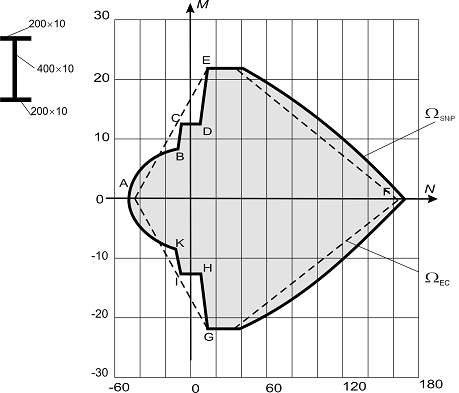
Figure 2. Load-bearing
capacity area of a steel section:
ΩSNiP – according to
SP 16.13330; ΩEC –
according to EN 1993-1-1:2005
The boundary of the load-bearing capacity area ΩSNiP on the DEFGH section is defined by the strength condition under the combined action of tension and bending, on the CD and IH sections – by the condition of stability of in-plane bending, and on the IKABC section – by the condition of stability out of the bending moment plane.
The non-convexity of the boundary of the load-bearing capacity area ΩSNiP on the IKABC section is related to the change in the type of dependence of the coefficient c on the value of the relative eccentricity m. This coefficient is included in the condition for checking the stability out of the plane of bending of a bar under bending and compression. The graphs с = с(mх) for three values of the effective length of the considered bar out of the bending plane are shown in Fig. 3, which shows a characteristic break at the value of the relative eccentricity mх = 10, where the function с(mх) changes from a linear to a hyperbolic one. The indicated break corresponds to the points K and B of the load-bearing capacity area ΩSNiP (Fig. 2).
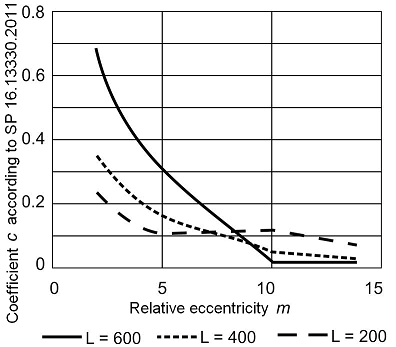
Figure 3. Dependence of the coefficient c on the relative eccentricity m
It should be noted that the nonconvexity of the IKABC section of the load-bearing capacity area ΩSNiP does not appear when the element has small out-of-plane slenderness, in spite of the fact that the break in the curveс = с(m) does not disappear, but for such design cases the condition of stability out of the bending moment plane is not determinative.
The configuration of the CDE and IHG sections of the load-bearing capacity area ΩSNiP is determined by the codes specifying that the stability of in-plane bending of a bar should be checked only at the values of the relative eccentricity mх > 20, when the stability check of such a bar has to be performed as for a flexural member. Sections of the boundary DC and JK of the load-bearing capacity area ΩSNiP correspond to these values (Fig. 2).
EN 1993-1-1:2005. Eurocode 3. Design of Steel Structures
The dashed line in Fig. 2 shows the load-bearing capacity area ΩЕС of a cross-section calculated according to the requirements of EN 1993-1-1:2005. The load-bearing capacity area of this section is convex, because the section operates within the limits of elastic deformation of steel.
Fig. 4 shows the load-bearing capacity area of a steel I-beam with a 800×10 mm web and 360×20 mm and 240×20 mm flanges generated in accordance with the requirements of EN 1993-1-1:2005. Here the nonconvexity of the load-bearing capacity area of the section is related to the requirements of EN 1993-1-1: 2005, concerning the classification of sections. In the stress state corresponding to the appearance of compressive stresses in one of the flanges, the section ceases to be classified as a section of the 2nd class (plastic deformations of steel, calculation using the plastic moment of resistance) and passes into the third class of sections (elastic deformations of steel, calculation using the elastic moment of resistance). The jumps AB and CD correspond to these transitions. A similar jump-like change in the boundary of the load-bearing capacity area can occur at the transition of the section from the 3rd class to the 4th one.
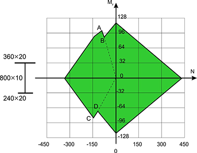
Figure 4. Load-bearing capacity area of a steel section according to EN 1993-1-1
The number of examples could be increased, but the ones given here indicate a very real situation when the load-bearing capacity area can turn out to be non-convex. As the analysis shows, in many cases there are some inconsistencies in the formulation of requirements for the bar elements of load-bearing structures, due most likely to insufficient adjustment of the formulations themselves.
The origin of such inconsistencies is related to the fact that the traditional approach based on the manual calculation generated all sorts of “simplifications”, which allowed to skip some checks or to replace the general case with a certain particular case (as at m < 20 for steel elements under bending and compression).
Moreover, the use of “logical switches” that change rules without an exact physical basis leads to an abrupt change in the algorithm, as in the classification of cross-sections in the Eurocode. Modern technologies enable to detect such inaccuracies and determine ways to improve the codes.
Dangers related to the nonconvexity of the load-bearing capacity area point to the necessity of analyzing the closeness of the set of the specified combinations of forces to the section of the boundary of the load-bearing capacity area, where the property of nonconvexity is manifested.
An almost identical analysis can be performed using additional tools
provided by SCAD Office. The following
buttons are provided for the analysis of problems related to the non-convexity
of the load-bearing capacity area: 
 . They enable to perform the following operations:
– if the
forces are specified, clicking this button will draw the entire set of
given combinations of forces as points corresponding to the projections
of the variants of combinations of forces on the plane of the selected
pair of forces (Fig. 5).
– drawing
a convex hull of the points specified above, i.e. an entire set of points
which may result from a linear combination of specified forces, including
their incomplete values.
Despite the fact that these combinations were not subjected to a direct check, in the case when the convex hull of loadings does not leave the load-bearing capacity area of the section, it can be ensured that the various loadings combined from the basic ones are not dangerous.
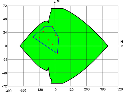
Figure 5. Given (basic) loadings and their convex hull, combined with the load-bearing capacity area of the section
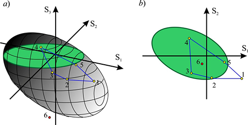
Figure 6. Illustration of possible design situations
It should be noted that the considered mechanism is a powerful tool for analyzing loading conditions, but it should be used carefully.
The load-bearing capacity area of a section is a body in the six-dimensional space of internal forces (with the coordinates N, My, Qz, Mz, Qy, T). The load-bearing capacity area is a section of the given body by a plane, and the point corresponding to the set of forces is the projection onto this plane. If the point corresponding to a certain set of forces lies within the load-bearing capacity area, it does not follow from this that all the requirements of the codes are satisfied. This is due, for example, to the fact that when generating the load-bearing capacity area (interaction curves), the restrictions of the limit slenderness are ignored (these restrictions do not depend on forces), and a situation may occur when the point belongs to the load-bearing capacity area of the section (lies in the “green area”), but the calculation will show Kmax > 1.
When operating only with two-dimensional orthogonal projections of the load-bearing capacity area, it is possible to “see” the projections of some points (combinations of internal forces) belonging to this area (for which the maximum utilization factor of restrictions does not exceed one Kmax < 1) as displayed outside the projection boundary of the load-bearing capacity area (as, for example, point 1 in Fig. 6). This can happen in the case when the Seismic checkbox is checked for the specified set of combination of internal forces, and as a result the service factor mcr > 1 was used in the calculation. And the generation of the load-bearing capacity area (interaction curves) is performed without taking into account factor mcr. A more complicated situation can arise when analyzing the interaction curves for reinforced concrete structures, since different sets of forces (points) may have different coefficients of duration.
There may also be an erroneous “vision” of a different kind, when the projection of the point lies within the boundaries of the projection of the load-bearing capacity area, and the point itself does not belong to the area (see, for example, point 6 in Fig. 6).
In order to identify such situations, the projections of the points in which the utilization factor of restrictions exceeds one, are displayed in red on the projections of the load-bearing capacity area, otherwise they are displayed in green.
In the program the Interaction Curves
tab has a button  , which enables to generate a surface
in 3D where Kmax=1
for the triple of internal forces and moments selected by the user (for
example, My-Mz-N). Clicking this button invokes
the dialog box, where you can select which force corresponds to a certain
coordinate axis (XYZ).
, which enables to generate a surface
in 3D where Kmax=1
for the triple of internal forces and moments selected by the user (for
example, My-Mz-N). Clicking this button invokes
the dialog box, where you can select which force corresponds to a certain
coordinate axis (XYZ).
Clicking the Apply button will start the calculation which can be aborted by clicking the Cancel button. Once the calculation is completed, the image of the interaction surface will appear.
Controls in the left side of the window enable to
In order to change the color or font, double click on the respective cell and select the parameters.
The Wireframe model checkbox enables to obtain an image of the surface in the form of a wireframe.
Right-clicking invokes the context menu where you can select a projection.
The following operations with the mouse can be performed in the program:
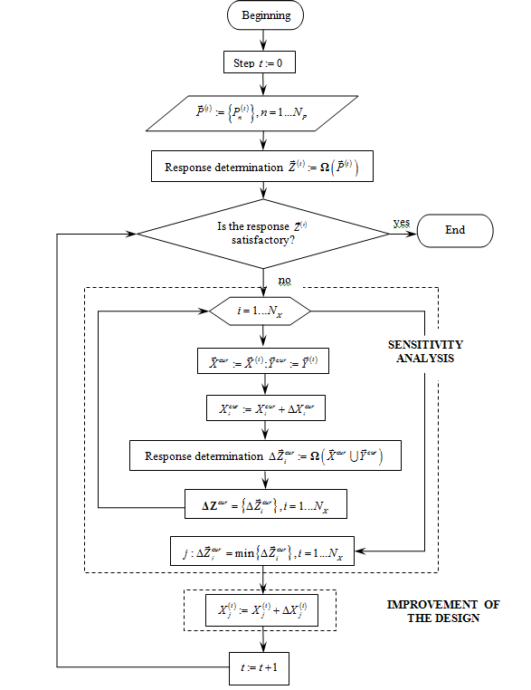
The software implementation of the automatic selection of the unknown parameters of the given type of the joint structure has been reduced to the problem of making a decision on the basis of the analysis of a mathematical model of the joint structure. Below you will find some additional commentaries given in order to define a number of principles for decision making, which are implemented in the software and thus have to be taken into account by the users.
A final combination of internal (integrated) parameters was determined for each group of joints (column bases, beam splices, beam-to-column joints) \( \vec{{P}}=\left\{ {P_{n} } \right\}, \quad n=\overline {1,N_{P} } \). A set of controlled parameters \( \vec{{X}}=\left\{ {X_{i} } \right\}\subset \vec{{P}}, \quad i=\overline {1,N_{X} } \) and a set of subordinated parameters \( \vec{{Y}}=\left\{ {Y_{j} } \right\}\subset \vec{{P}},j=\overline {1,N_{Y} } , \quad \vec{{P}}=\vec{{X}}\cup \vec{{Y}} \) were distinguished among them. A specific feature of the design object (structural joint) is that its controlled parameters can be both independent and dependent on each other (for example, the end-plate thickness and the diameter of bolts in end-plate joints), and it is difficult to represent this dependence analytically, while the subordinated parameters can always be determined (calculated) unambiguously depending on the values of the controlled parameters, \( \vec{{Y}}={\rm {\bf \Theta }}\left\{ {\vec{{X}}} \right\}. \). For example, if we consider an erection beam splice with end-plates, the end-plate thickness, the diameter of bolts and the number bolt rows will be the controlled parameters, and the other parameters of the software interface will be the subordinated ones.
|
A flowchart of the decision making algorithm when selecting the parameters of the structural joint |
The parameters of state (output) have been also included in the mathematical model of the structural joint \( \vec{{Z}}=\left\{ {Z_{k} } \right\},k=\overline {1,N_{Z} } , \quad k=\overline {1,N_{Z} } \) – values which characterize the integral properties of the design object, they can only be calculated: \( \vec{{Z}}:={\rm {\bf \Omega }}\left( {\vec{{P}}} \right) \), but they cannot be directly varied. They are unambiguously dependent on the values of the internal parameters of the design object (structural joint). The utilization factors of restrictions of the load-bearing capacity of the structural elements of the joint defined by the standard requirements were considered as the parameters of state.
The selection of a certain design of the joint is the determination of the certain values of the whole set of its internal parameters.
When the decision was made, the values of the internal parameters varied within certain limits defined by the system of inequalities:
\[ \left\{ {\begin{array}{l} {\rm {\bf \varphi }}_{1} \left( {\vec{{P}}} \right)\le 0,{\rm {\bf \varphi }}_{1} =\left\{ {\psi_{\kappa } ,\phi_{\eta } } \right\}; \\ {\rm {\bf \varphi }}_{2} \left( {\vec{{Z}}\left( {\vec{{P}}} \right)} \right)\le 0,{\rm {\bf \varphi }}_{2} =\left\{ {\psi _{\kappa } ,\phi_{\eta } } \right\}; \\ \end{array}} \right.\kappa =\overline {1,N_{EC} } ,\eta =\overline {1,N_{IC} } \]
which included:
The automatic determination of the unknown values of the internal parameters of the joint design is implemented as a targeted iterative improvement of a certain initial joint design toward the fulfillment of a set of constraints by bearing capacity taking into account the structural constraints and assortment constraints. The iterative improvement of the design is performed on the basis of the analysis of its sensitivity with respect to the variation of the controlled parameters in the structure of the joint. The response of the system (values of the utilization factors of restrictions of the load-bearing capacity) is evaluated at each variation of a certain controlled parameter. Finally, the decision to increase the controlled parameter the variation of which has provided the “best” (in terms of satisfying the restrictions of the bearing capacity) design of the joint structure is made.
Assortment constraints are taken into account both on the stage of determining the starting values of the internal parameters of the joint structure and on the stage of their variation (increasing) which is provided strictly according to the assortments of rolled structural steels and plates.
Structural constraints (which include the conditions of manufacturing structural members, constraints imposed on the mutual arrangement of members by the possibility of making welded and bolted connections, conditions of weldability of members of different thickness, and others) were described by the functional relationships which connected the subordinated parameters of the joint structure with the controlled ones.
A flowchart of the decision making algorithm is given in the figure.
In cases when it is impossible to obtain a joint design for the initial data specified by the user, which would comply with building codes, the application performs an analysis of the load-bearing capacity of the joint design, outputs the results of the analysis, and gives recommendations on how to improve its load-bearing capacity.