|
|
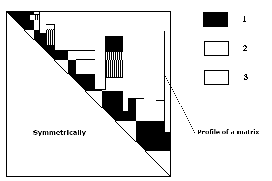
Figure 1. The profile of a matrix. (1) nonzero elements, (2) zero elements filled during the matrix decomposition, (3) zero elements not filled during the matrix decomposition. |
|
Once a given structure is represented as a finite element model, the problem of determining nodal displacements is reduced to the solution of a system of linear algebraic equations:
KZ = F, |
(1) |
where K is a symmetric N×N matrix. It should be noted that matrix K is usually positive definite and contains a considerable number of zero elements (i.e., it is a sparse matrix);
F is the N×k matrix of right hand side (loadings), where k is the number of loadings;
Z is the unknown k×N matrix of displacements.
There are both direct and iterative methods for solving systems of linear algebraic equations. The direct methods are a powerful tool for solving systems of linear algebraic equations with sparse matrices if there is an efficient way to order the unknowns and thus reduce the fill-in in the matrix factorization. The advantages of these methods are that they are less sensitive to the ill-conditioning of systems of equations, enable to detect modeling mistakes that lead to a dimensional instability of the design model, and that the computation time does not depend much on the right hand side if the latter is relatively small.
Iterative methods for solving systems of linear algebraic equations are widely used to study large-scale problems of solid mechanics. They are particularly useful in cases when a lot of fill-ins appear in the structure of the adjacency graph levels, which drastically slows the performance of the direct methods. The iterative methods are usually used in cases when the matrix of the system of equations is positive definite.
The most popular direct methods used in FEM software include a profile method based on Gaussian exclusions, and a frontal method. In the first case the matrix of governing equations is fully formed before solving these equations (see Fig. 1); in the second case groups of equations usually containing unknowns of a single node are formed in RAM. The stiffness matrix of the system is not assembled explicitly; the stiffness matrices of the elements with the degrees of freedom included in the given group are gradually added instead. Once the new front is assembled, i.e. all its adjoining elements are included in the assembly, unknowns the numbers of which do not coincide with those of the front equations will be at once subjected to the Gaussian exclusion procedure. As a result, the Gaussian exclusion is performed in a dense (frontal) matrix of relatively small size that consists of a fully assembled part of the equations and an incomplete one. In the course of the solution, the front moves along the nodes of the FEM model. The efficiency of the multifrontal method is usually an order of magnitude greater than that of the modified Gaussian algorithm.
Arrangement of the order of the equation exclusion (profile method) or of the inclusion of the finite elements in the stiffness matrix assemblage (frontal method) aimed at the reduction of fill-ins is usually performed taking into account the structure of the stiffness matrix fill-ins. Here and further, a fill-in will refer to a nonzero element that appears in the matrix during the factorization in the place of an original zero element (see Fig. 1). The number of fill-ins greatly affects the efficiency of both methods for solving linear algebraic equations.
Several renumbering methods are implemented in SCAD, e.g., the reverse Cuthill-McKie algorithm, the factor tree method, the method of nested sections, the algorithm of parallel sections, the METIS algorithm, the Sloane algorithm, the minimum degree algorithm, etc. These methods and their comparative characteristics are described in the literature on the subject. The user is authorized to select a renumbering method, because the efficiency of an algorithm greatly depends on the structure of a particular matrix К, and the problem of determining the optimal renumbering of the degrees of freedom belongs to “difficult problems” (NP-complete) [19], [26], [27].
It is recommended to use a high-performance parallel solver PARFES for multi-core computers, which enables to calculate large problems much faster.
If any of the SCAD solvers is used and the process of triangular decomposition of matrix K makes one of the governing elements equal to zero, i.e. matrix K is found to be degenerate, which indicates that the structure is unstable, then an additional unstressed constraint is automatically imposed to make the system stable. The user receives information on the node numbers and the types of degrees of freedom involved in this additional constraining. It should be noted that the degenerate character of the matrix is not identified by an exact equality of the governing element to zero, but rather by a “nearly zero” number appearing on the main diagonal. The threshold for this “nearly zero” magnitude (a solution accuracy parameter) is one of the properties the user is authorized to set up.
|
|
Figure 1. The profile of a matrix. (1) nonzero elements, (2) zero elements filled during the matrix decomposition, (3) zero elements not filled during the matrix decomposition. |
|
When a message about additionally imposed constraints appears in the log file, we recommend you to review your design model carefully and find out the reason for the dimensional instability of the structure. It might turn out that the system is formally stable, but its elements have such parameters of rigidity that it is defined as “almost unstable”. Then in order to perform the analysis you might have to solve the problem again with another solution accuracy parameter.
An additional service function is a system solution check (1). If there is a message that the solution error is too large (this is usually due to an ill-conditioned matrix K), you should carefully analyze the nodal displacements and make sure that the obtained solution is acceptable from the engineering standpoint. The ill-conditionality is usually caused by an improper structural design (for example, the system is “almost unstable”) or its incorrect idealization.