Principal and Equivalent Stresses

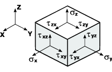
Figure 1. Stress components

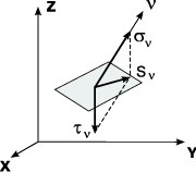
Figure 2. Stresses on an arbitrary plane

Let’s outline the fundamental principles of the stress theory usually considered in the course of the theory of elasticity or the strength of materials.

If you select an elementary volume in the form of an infinitesimally small parallelepiped from the body in the vicinity of a certain point (Fig.1), the environmental action on it can be replaced by the stresses the components of which act on the faces of the parallelepiped.

According to the law of pairing of shear stresses

\[ \tau_{xy} =\tau_{yx} , \quad \tau_{yz} =\tau_{zy} , \quad \tau_{zx} =\tau_{xz} . \]

(1)

In the general case there are only six independent stress components in a point which form a symmetric stress tensor

\[ T_{\sigma } =\left[ {{\begin{array}{*{20}c} {\sigma_{x} } & {\tau_{xy} } & {\tau_{xz} } \\ {\tau_{xy} } & {\sigma_{y} } & {\tau_{yz} } \\ {\tau_{xz} } & {\tau_{yz} } & {\sigma_{z} } \\ \end{array} }} \right]. \]

(2)

Normal stress σ_ν and shear stress τ_ν (Fig. 2) with the resultant S_ν act on an arbitrarily oriented plane passing through the same point the normal to which ν has direction cosines l, m, n with the axes x, y, z. The projections of this resultant on the coordinate axes S_νx, S_νy, S_νz are related to the stress components by the equilibrium conditions (Cauchy’s formula):

\[ \left. {\begin{array}{l} S_{\nu x} =\sigma_{x} l+\tau_{xy} m+\tau_{xz} n \\ S_{\nu y} =\tau_{xy} l+\sigma_{y} m+\tau_{yz} n \\ S_{\nu z} =\tau_{xz} l+\tau_{yz} m+\sigma_{z} n \\ \end{array}} \right\} \]

(3)

There are such three mutually perpendicular planes on which there are no shear stresses. Principal stresses σ₁, σ₂ and σ₃ (σ₁ ≥ σ₂ ≥ σ₃) act on these so-called principal planes. It is also known that the principal stresses have extreme properties, i.e. the resulting stress on any plane S_ν ≤ σ₁ and S_ν ≥ σ₃.

The direction cosines l_k, m_k and n_k of the normals to the principal planes ν_k are determined by solving the system of equations:

\[ \left\{ {\begin{array}{l} (\sigma_{x} -\sigma_{k} )l_{k} +\tau_{xy} m_{k} +\tau_{xz} n_{k} =0; \\ \tau_{xy} l_{k} +(\sigma_{y} -\sigma_{k} )m_{k} +\tau_{yz} n_{k} =0; \\ \tau_{xz} l_{k} +\tau_{yz} m_{k} +(\sigma_{z} -\sigma_{k} )n_{k} =0; \\ \end{array}} \right. \]

(4)

a nonzero solution of which exists when its determinant is equal to zero.

And \( l_{k}^{2} +m_{k}^{2} +n_{k}^{2} =1 \).

It follows from (4) that the principal stresses σ_k(k=1,2,3) are the roots of the cubic equation

\[ det\left[ {{\begin{array}{*{20}c} {\sigma_{x} -\sigma } & {\tau_{xy} } & {\tau_{xz} } \\ {\tau_{xy} } & {\sigma_{y} -\sigma } & {\tau_{yz} } \\ {\tau_{xz} } & {\tau_{yz} } & {\sigma_{z} -\sigma } \\ \end{array} }} \right]=0. \]

(5)

Expanded form of the equation (5):

\[ \sigma^{3}-I_{1} (T_{\sigma } )\sigma^{2}-I_{2} (T_{\sigma } )\sigma -I_{3} (T_{\sigma } )=0, \]

(6)

Its coefficients are invariants (i.e. they do not depend on the selected coordinate system). The first invariant \( I_{1} (T_{\sigma } )=\sigma_{x} +\sigma_{y} +\sigma_{z} \) is equal to three times the average stress (hydrostatic pressure) σ₀.

The direction of the principal planes can be defined not only by the nine direction cosines but also by the three Euler angles (precession angle ψ, nutation angle θ and the pure rotation angle φ). Any plane parallel to the coordinate plane (XOY, XOZ or YOZ) can be set to any position with their help.

The Lode-Nadai coefficient is used to characterize the stress-strain state (SSS).

\[ \mu_{0} =2\frac{\sigma_{2} -\sigma_{3} }{\sigma_{1} -\sigma_{3} }-1, \]

It takes values μ₀ = 1 at pure compression, μ₀ = 0 at pure shear, μ₀= -1 at pure tension.

When outputting the results of the calculation the stress tensor (2) in the general case has the following form

\[ T_{\sigma } =\left[ {{\begin{array}{*{20}c} {\sigma_{x} } & {T_{xy} } & {T_{xz} } \\ {T_{xy} } & {\sigma_{y} } & {T_{yz} } \\ {T_{xz} } & {T_{yz} } & {\sigma_{z} } \\ \end{array} }} \right] \]

(7)