Cube under the Constant Stresses throughout the Volume

Objective: Check of the obtained values of the constant stresses throughout the volume of the cube at an irregular coarse finite element mesh.
Initial data files:
|
File name |
Description |
|---|---|
|
Design model with the elements of type 32 |
|
|
Design model with the elements of type 34 |
|
|
Design model with the elements of type 36 |
|
|
Design model with the elements of type 37 |
Problem formulation: The unit isotropic cube is subjected to the displacements of the external surfaces providing the conditions of the constant stresses throughout the volume. Check that the conditions of constant normal σx, σy, σz and tangential τxy, τxz, τyz stresses throughout the volume are provided.
References: R. H. Macneal, R. L. Harder, A proposed standard set of problems to test finite element accuracy, North-Holland, Finite elements in analysis and design, 1, 1985, p. 3-20.
Initial data:
| E = 1.0·106 kPa | - elastic modulus of the plate material; |
| ν = 0.25 | - Poisson’s ratio; |
| a = 1.00 m | - side of the cube; |
| Boundary conditions: | |
| u = 10-3∙(2∙x + y + z)/2 | - displacement of the external surfaces along the X axis of the global coordinate system; |
| v = 10-3∙(x + 2∙y + z)/2 | - displacement of the external surfaces along the Y axis of the global coordinate system; |
| w = 10-3∙(x + y + 2∙z)/2 | - displacement of the external surfaces along the Z axis of the global coordinate system; |
Location of internal nodes of the finite element mesh:
|
Numbers of nodes in the Figure 1 |
x |
y |
z |
|---|---|---|---|
|
1 |
0.35 |
0.35 |
0.35 |
|
2 |
0.75 |
0.25 |
0.25 |
|
3 |
0.85 |
0.85 |
0.15 |
|
4 |
0.25 |
0.75 |
0.25 |
|
5 |
0.35 |
0.35 |
0.65 |
|
6 |
0.75 |
0.25 |
0.75 |
|
7 |
0.85 |
0.85 |
0.85 |
|
8 |
0.25 |
0.75 |
0.75 |
Finite element model: Design model – general type system. Four design models are considered:
Model 1 - 42 four-node pyramid elements of type 32. Boundary conditions are provided by imposing constraints on the nodes of the external surfaces of the cube in the directions of the degrees of freedom X, Y, Z and their displacement in accordance with the specified values u, v, w. Number of nodes in the model – 16.
Model 2 - 14 six-node isoparametric solid elements of type 34. Boundary conditions are provided by imposing constraints on the nodes of the external surfaces of the cube in the directions of the degrees of freedom X, Y, Z and their displacement in accordance with the specified values u, v, w. Number of nodes in the model – 16.
Model 3 - 7 eight-node isoparametric solid elements of type 36. Boundary conditions are provided by imposing constraints on the nodes of the external surfaces of the cube in the directions of the degrees of freedom X, Y, Z and their displacement in accordance with the specified values u, v, w. Number of nodes in the model – 16.
Model 4 - 7 twenty-node isoparametric solid elements of type 37. Boundary conditions are provided by imposing constraints on the nodes of the external surfaces of the cube in the directions of the degrees of freedom X, Y, Z and their displacement in accordance with the specified values u, v, w. Number of nodes in the model – 48.
Results in SCAD
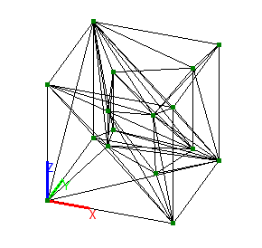
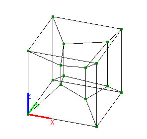
Model 1. Design and deformed models
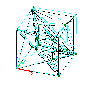
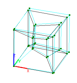
Model 2. Design and deformed models
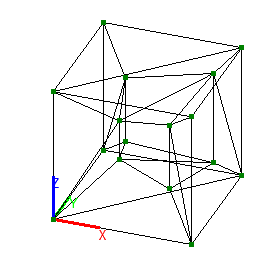
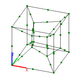
Model 3. Design and deformed models
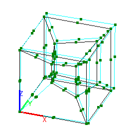
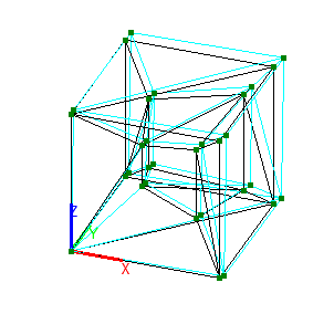
Model 4. Design and deformed models
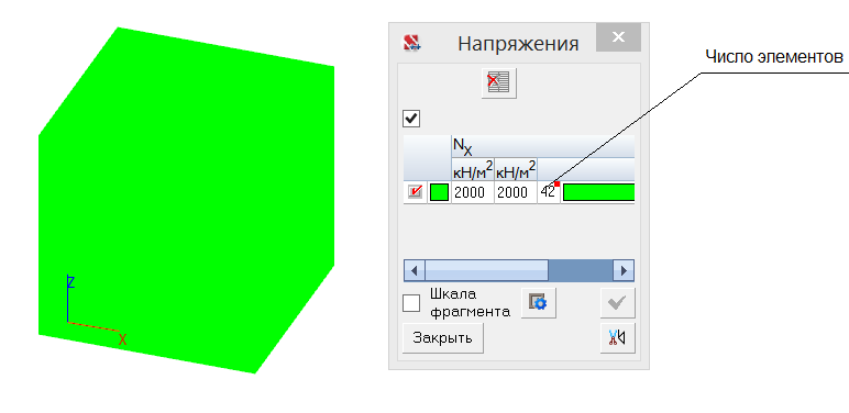
Values of normal stresses for all models σx, σy σz (kN/m2)
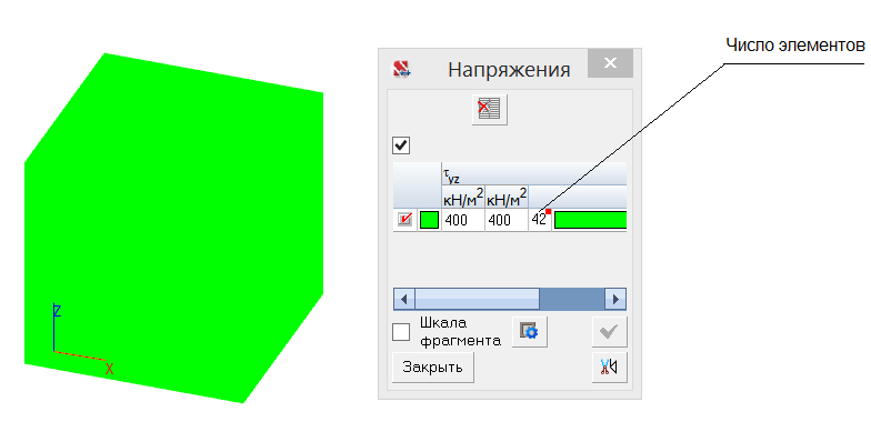
Values of tangential stresses for all models τxz, τxy, τyz (kN/m2)
Comparison of solutions:
|
Model |
Parameter |
Theory |
SCAD |
Deviation, % |
|---|---|---|---|---|
|
1-4 |
Normal stresses σx, kN/m2 |
2000 |
2000 |
0.00 |
|
Normal stresses σy, kN/m2 |
2000 |
2000 |
0.00 |
|
|
Normal stresses σz, kN/m2 |
2000 |
2000 |
0.00 |
|
|
Tangential stresses τxy, kN/m2 |
400 |
400 |
0.00 |
|
|
Tangential stresses τxz, kN/m2 |
400 |
400 |
0.00 |
|
|
Tangential stresses τyz, kN/m2 |
400 |
400 |
0.00 |
Notes: In the analytical solution the normal σx, σy, σz and tangential τxy, τxz, τyz stresses throughout the volume of the cube are determined according to the following formulas:
\[ \sigma_{x} =10^{-3}\cdot \frac{E}{1-2\cdot \nu }; \quad \sigma_{y} =10^{-3}\cdot \frac{E}{1-2\cdot \nu }; \quad \sigma_{z} =10^{-3}\cdot \frac{E}{1-2\cdot \nu }; \] \[ \tau_{xy} =10^{-3}\cdot \frac{E}{2\cdot \left( {1+\nu } \right)}; \quad \tau_{xz} =10^{-3}\cdot \frac{E}{2\cdot \left( {1+\nu } \right)}; \quad \tau_{yz} =10^{-3}\cdot \frac{E}{2\cdot \left( {1+\nu } \right)}. \]