Curvilinear Cantilever Beam with Concentrated Shear Forces at Its Free End

Objective: Check of the obtained values of the transverse displacements of the free end of a curvilinear cantilever beam subjected to concentrated shear forces.
Initial data files:
|
File name |
Description |
|---|---|
|
Design model with the elements of type 42 |
|
|
Design model with the elements of type 142 |
|
|
Design model with the elements of type 44 |
|
|
Design model with the elements of type 144 |
|
|
Design model with the elements of type 45 |
|
|
Design model with the elements of type 145 |
|
|
Design model with the elements of type 50 |
|
|
Design model with the elements of type 150 |
|
|
Design model with the elements of type 36 |
|
|
Design model with the elements of type 37 |
Problem formulation: The curvilinear isotropic cantilever beam of a rectangular cross-section is subjected to the concentrated shear forces Py, Pz (bending in and out of the plane of the longitudinal axis of the beam) applied at its free end. Check the obtained values of the transverse displacements Y, Z of the free end of the curvilinear cantilever beam from the respective actions.
References: R. H. Macneal, R. L. Harder, A proposed standard set of problems to test finite element accuracy, North-Holland, Finite elements in analysis and design, 1, 1985, p. 3-20.
Initial data:
| E = 1.0·107 kPa | - elastic modulus of the beam material; |
| ν = 0.25 | - Poisson’s ratio; |
| b = 0. 1 m | - width of the beam; |
| h = 0. 2 m | - height of the beam; |
| R = 4.22 m | - radius of the arc of the longitudinal axis of the beam; |
| α = π/2 rad | - central angle of the arc of the longitudinal axis of the beam; |
| Py = 1.0 kN | - value of the shear force acting along the height of the beam (in the plane of the longitudinal axis); |
| Pz = 1.0 kN | - value of the shear force acting along the width of the beam (out of the plane of the longitudinal axis). |
Finite element model: Design model – general type system. Ten design models with a trapezoidal finite element mesh are considered:
Model 1 - 12 three-node shell elements of type 42. Boundary conditions are provided by imposing constraints on the nodes of the clamped end of the beam in the directions of the degrees of freedom X, Y, Z, UX, UY, UZ. The concentrated shear Py, Pz forces are given in the form of two nodal forces (Py = 2∙0.5 kN, Pz = 2∙0.5 kN). Number of nodes in the model – 14.
Model 2 - 12 three-node shell elements allowing for shear of type 142. Boundary conditions are provided by imposing constraints on the nodes of the clamped end of the beam in the directions of the degrees of freedom X, Y, Z, UX, UY, UZ. The concentrated shear Py, Pz forces are given in the form of two nodal forces (Py = 2∙0.5 kN, Pz = 2∙0.5 kN). Number of nodes in the model – 14.
Model 3 - 6 four-node shell elements of type 44. Boundary conditions are provided by imposing constraints on the nodes of the clamped end of the beam in the directions of the degrees of freedom X, Y, Z, UX, UY, UZ. The concentrated shear Py, Pz forces are given in the form of two nodal forces (Py = 2∙0.5 kN, Pz = 2∙0.5 kN).. Number of nodes in the model – 14.
Model 4 - 6 four-node shell elements allowing for shear of type 144. Boundary conditions are provided by imposing constraints on the nodes of the clamped end of the beam in the directions of the degrees of freedom X, Y, Z, UX, UY, UZ. The concentrated shear Py, Pz forces are given in the form of two nodal forces (Py = 2∙0.5 kN, Pz = 2∙0.5 kN). Number of nodes in the model – 14.
Model 5 - 12 six-node shell elements of type 45. Boundary conditions are provided by imposing constraints on the nodes of the clamped end of the beam in the directions of the degrees of freedom X, Y, Z, UX, UY, UZ. The concentrated shear Py, Pz forces are given in the form of two nodal forces (Py = 2∙0.5 kN, Pz = 2∙0.5 kN). Number of nodes in the model – 39.
Model 6 - 12 six-node shell elements allowing for shear of type 145. Boundary conditions are provided by imposing constraints on the nodes of the clamped end of the beam in the directions of the degrees of freedom X, Y, Z, UX, UY, UZ. The concentrated shear Py, Pz forces are given in the form of two nodal forces (Py = 2∙0.5 kN, Pz = 2∙0.5 kN). Number of nodes in the model – 39.
Model 7 - 6 eight-node shell elements of type 50. Boundary conditions are provided by imposing constraints on the nodes of the clamped end of the beam in the directions of the degrees of freedom X, Y, Z, UX, UY, UZ. The concentrated shear Py, Pz forces are given in the form of two nodal forces (Py = 2∙0.5 kN, Pz = 2∙0.5 kN). Number of nodes in the model – 33.
Model 8 - 6 eight-node shell elements allowing for shear of type 150. Boundary conditions are provided by imposing constraints on the nodes of the clamped end of the beam in the directions of the degrees of freedom X, Y, Z, UX, UY, UZ. The concentrated shear Py, Pz forces are given in the form of two nodal forces (Py = 2∙0.5 kN, Pz = 2∙0.5 kN). Number of nodes in the model – 33.
Model 9 - 6 eight-node isoparametric solid elements of type 36. Boundary conditions are provided by imposing constraints on the nodes of the clamped end of the beam in the directions of the degrees of freedom X, Y, Z, UX, UY, UZ. The concentrated shear Py, Pz forces are given in the form of four nodal forces (Py = 4∙0.25 kN, Pz = 4∙0.25 kN). Number of nodes in the model – 28.
Model 10 - 6 twenty-node isoparametric solid elements of type 37. Boundary conditions are provided by imposing constraints on the nodes of the clamped end of the beam in the directions of the degrees of freedom X, Y, Z, UX, UY, UZ. The concentrated shear Py, Pz forces are given in the form of four nodal forces (Py = 4∙0.25 kN, Pz = 4∙0.25 kN). Number of nodes in the model – 80.
Results in SCAD
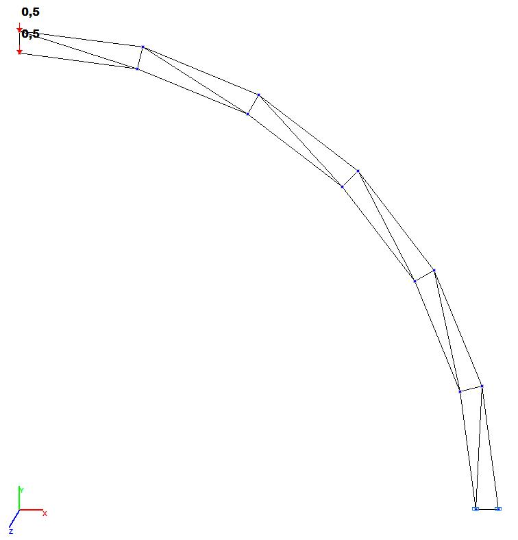
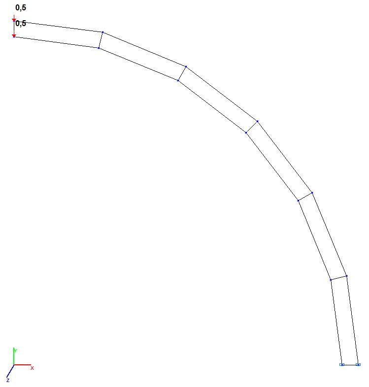
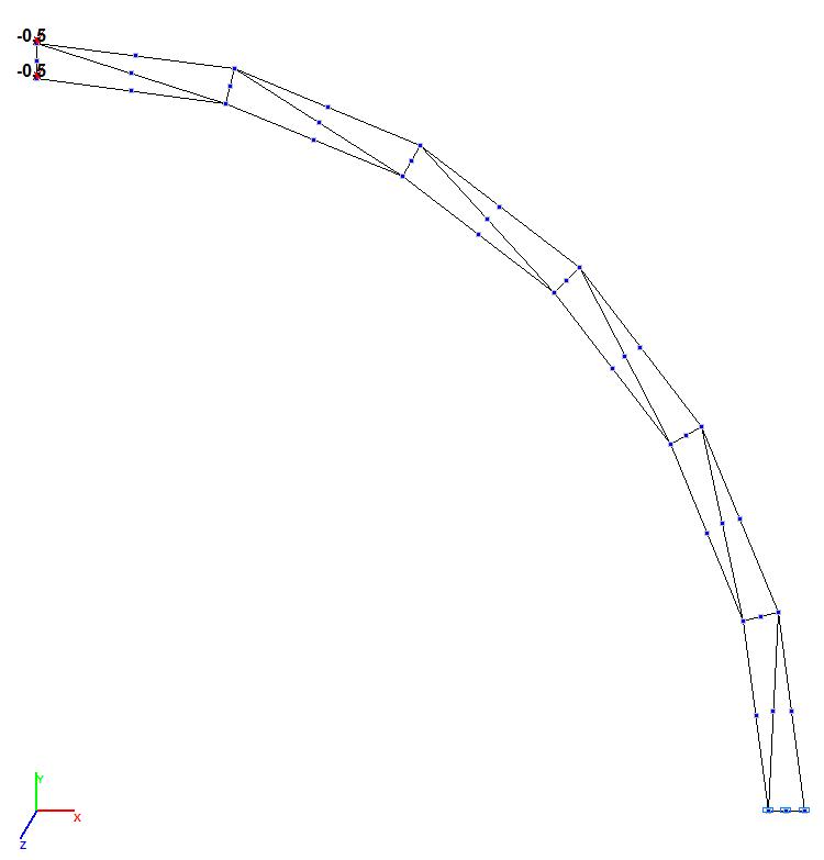
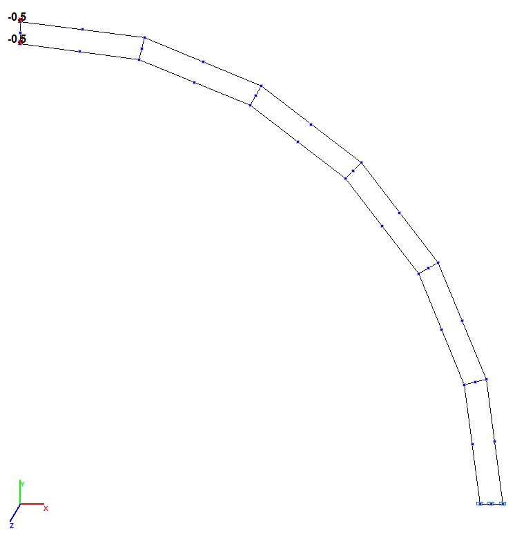
Models 1 and 2. Design model
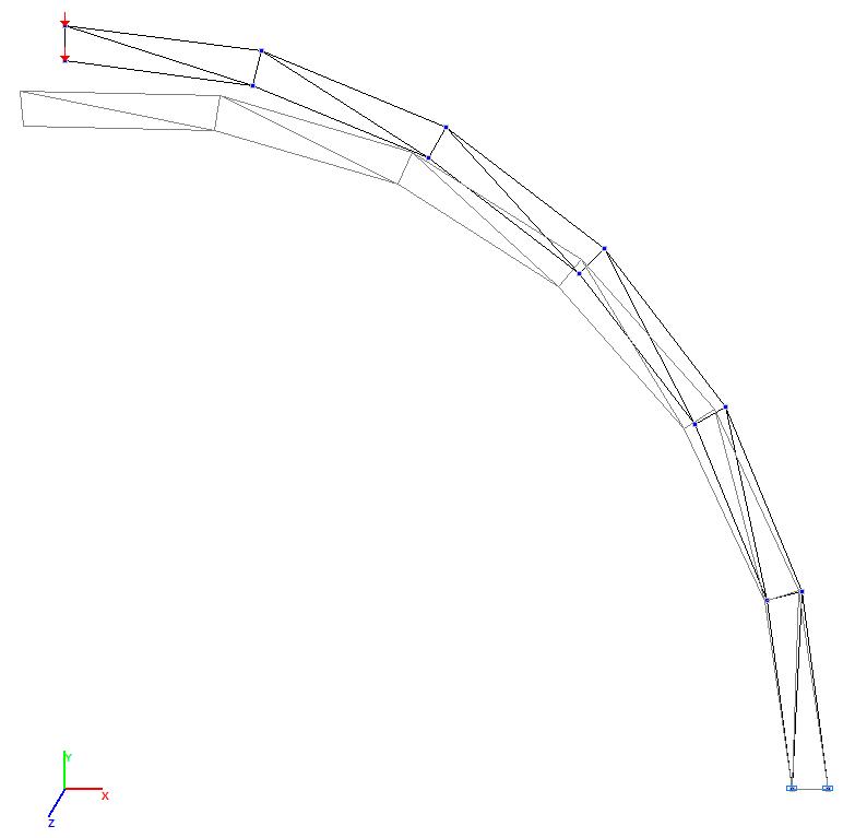
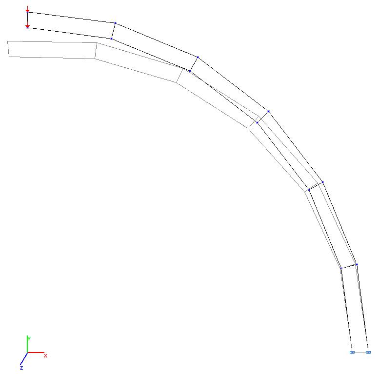
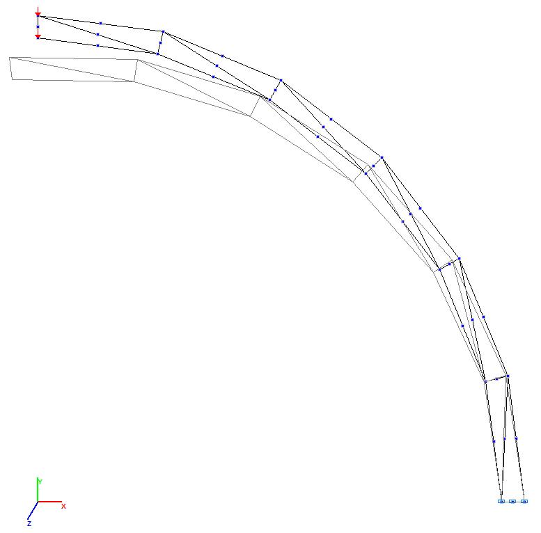
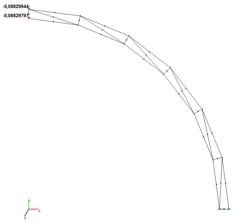
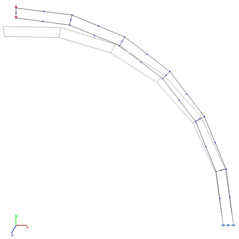
Models 1 and 2. Deformed model
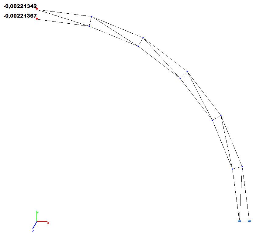
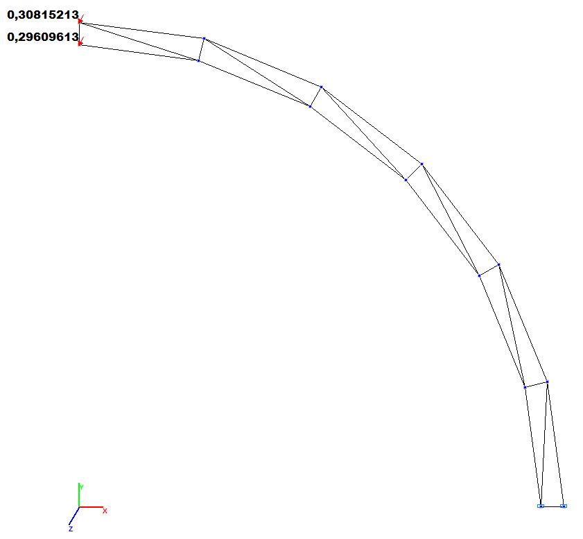
Model 1. Values of the transverse displacements Y, Z of the free end of the curvilinear cantilever beam (m, m)
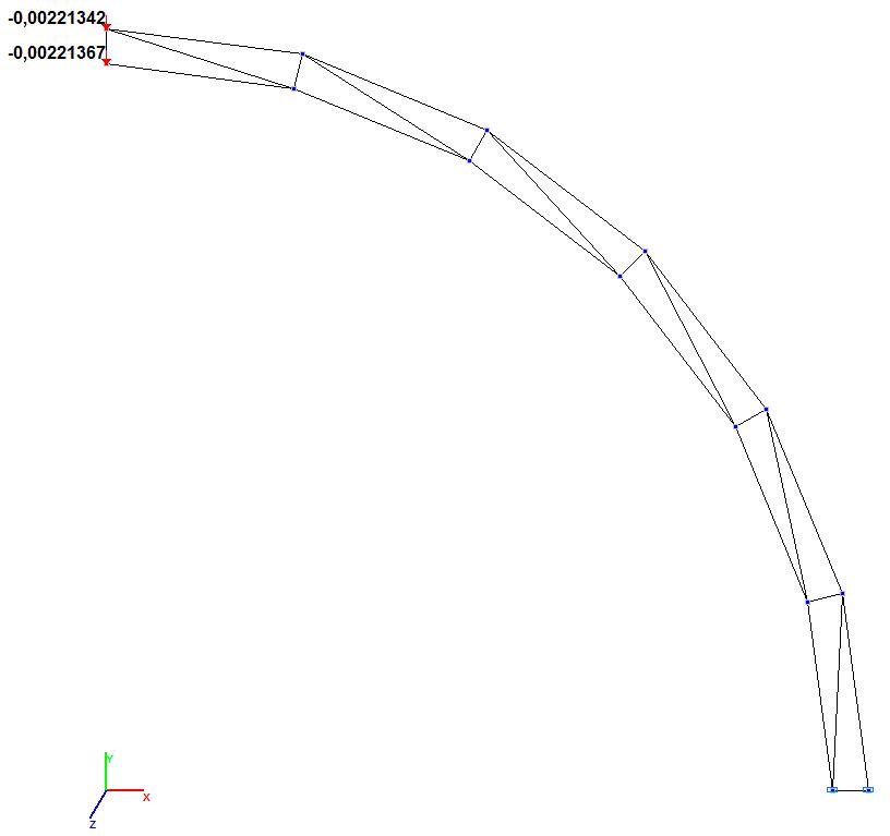
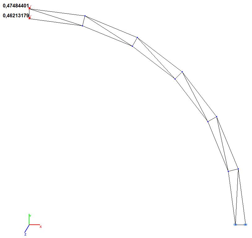
Model 2. Values of the transverse displacements Y, Z of the free end of the curvilinear cantilever beam (m, m)
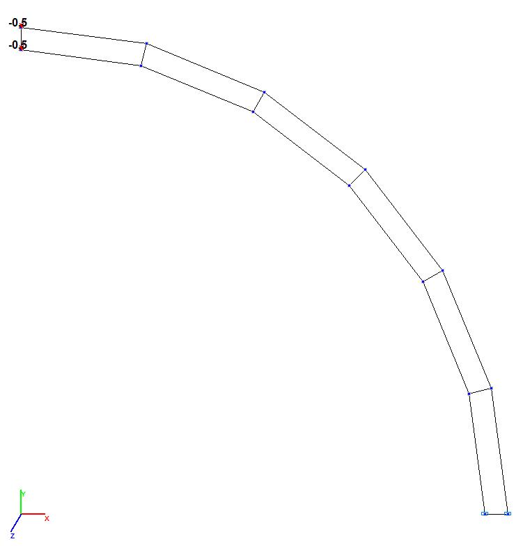
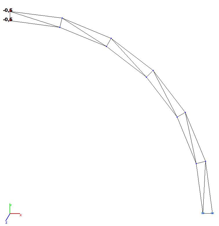
Models 3 and 4. Design model
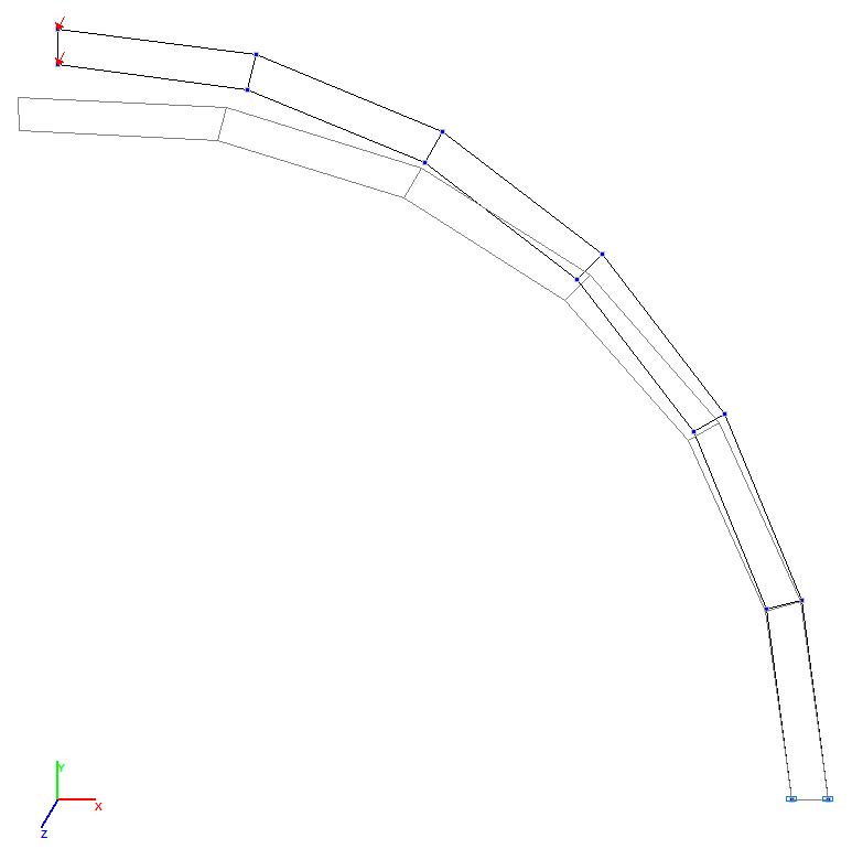
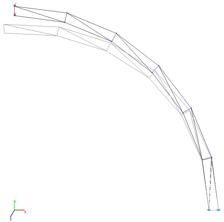
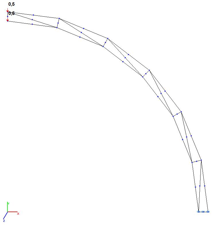
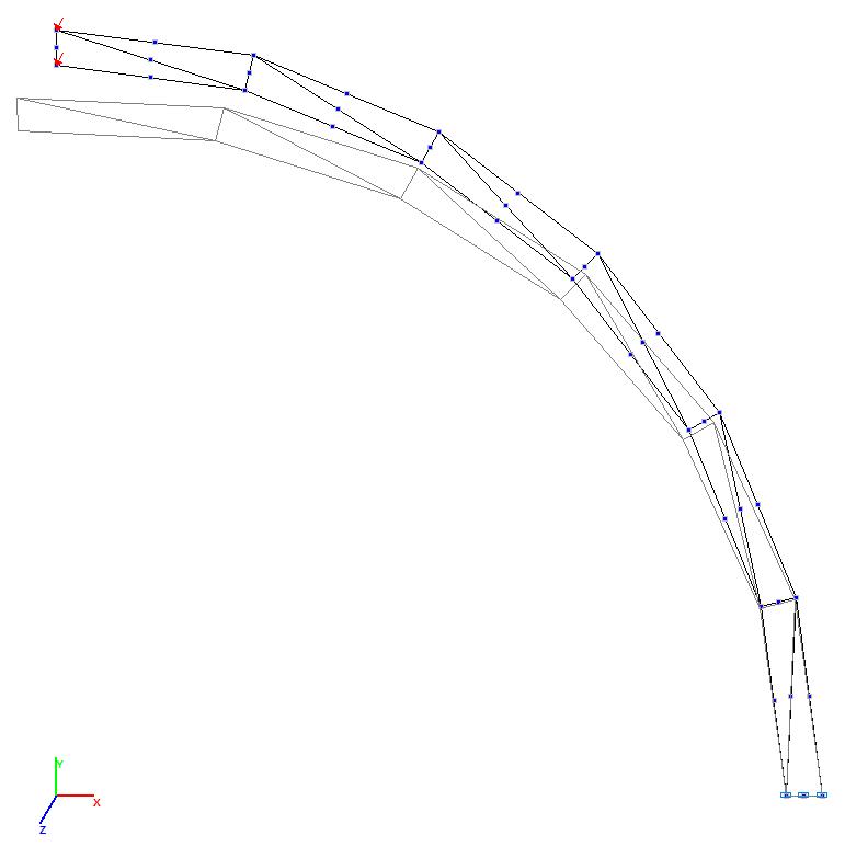
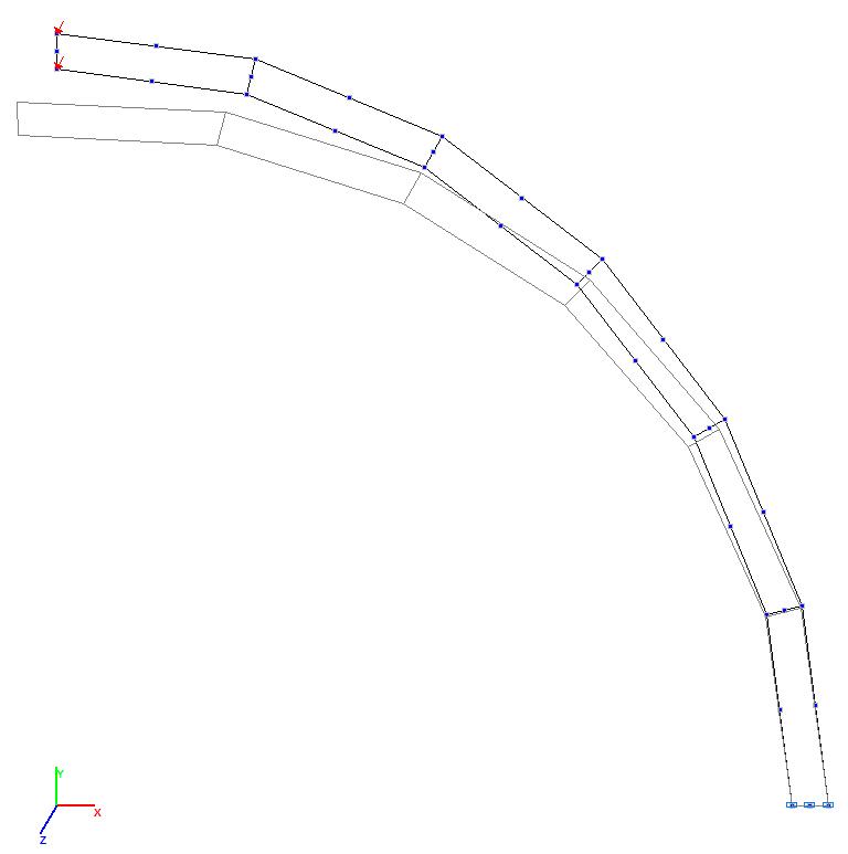
Models 3 and 4. Deformed model

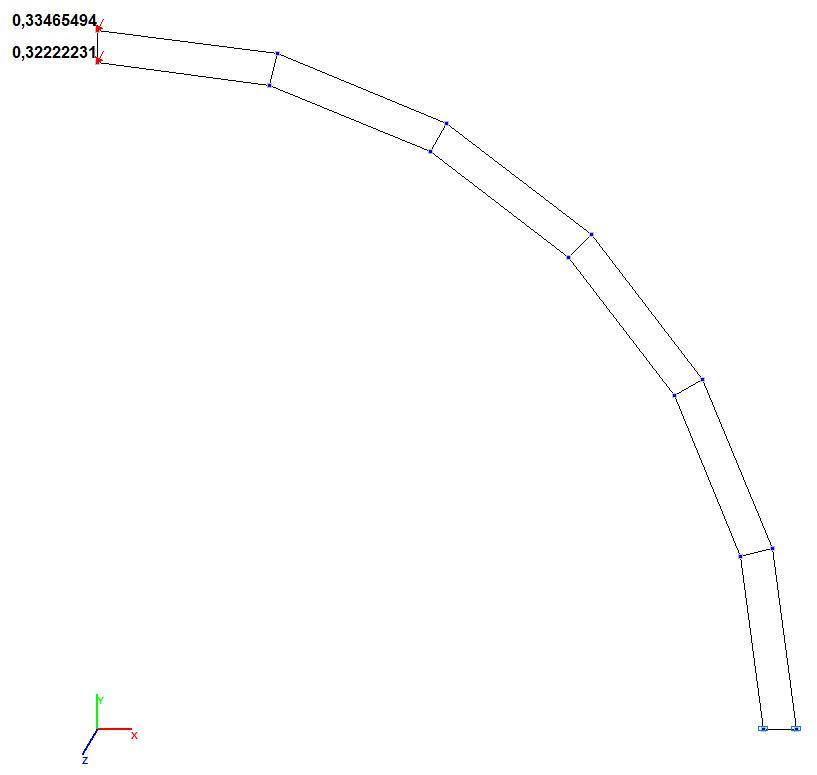
Model 3. Values of the transverse displacements Y, Z of the free end of the curvilinear cantilever beam (m, m)
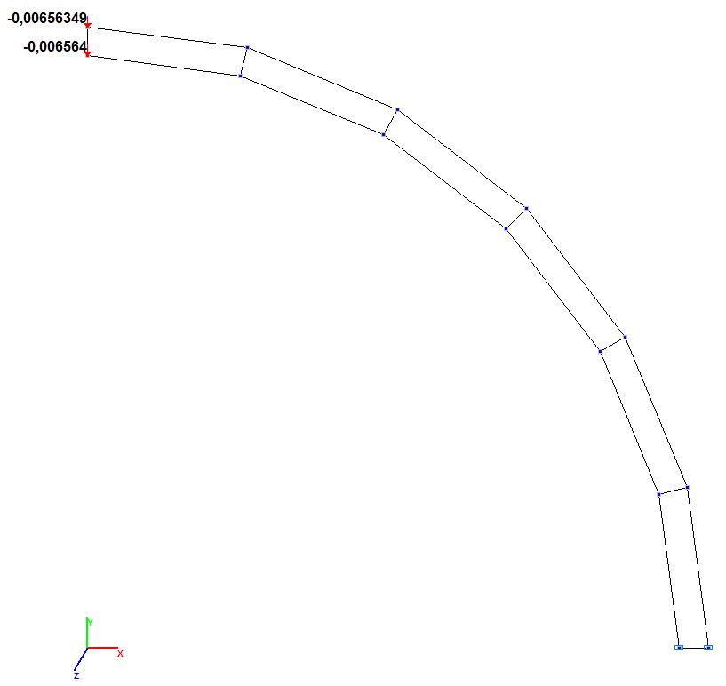
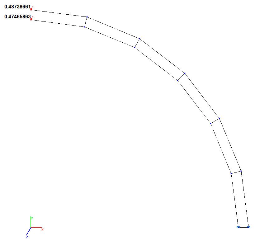
Model 4. Values of the transverse displacements Y, Z of the free end of the curvilinear cantilever beam (m, m)
Models 5 and 6. Design model
Models 5 and 6. Deformed model
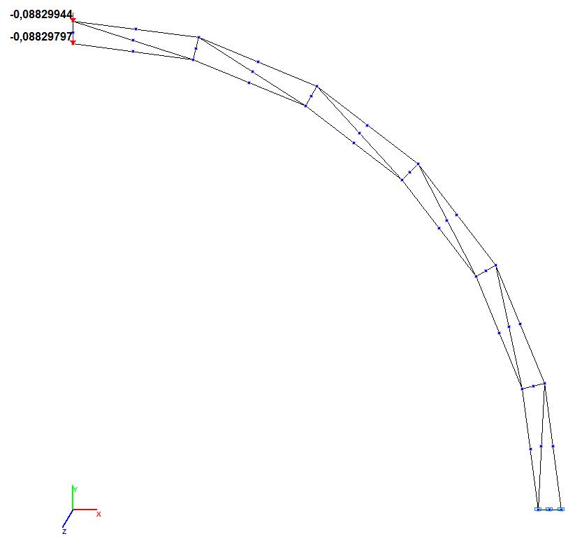
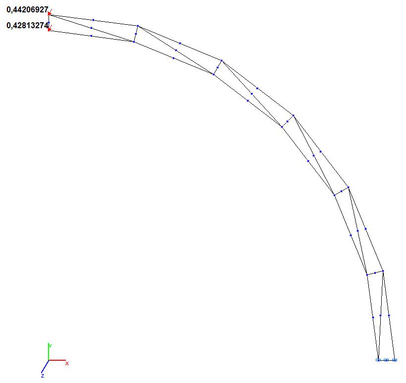
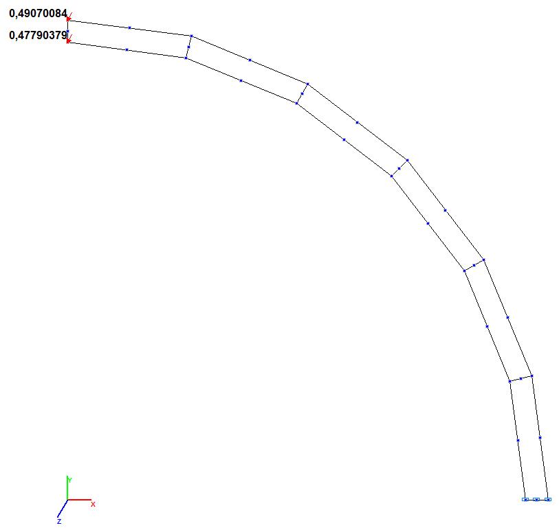
Model 5. Values of the transverse displacements Y, Z of the free end of the curvilinear cantilever beam (m, m)
Model 6. Values of the transverse displacements Y, Z of the free end of the curvilinear cantilever beam (m, m)
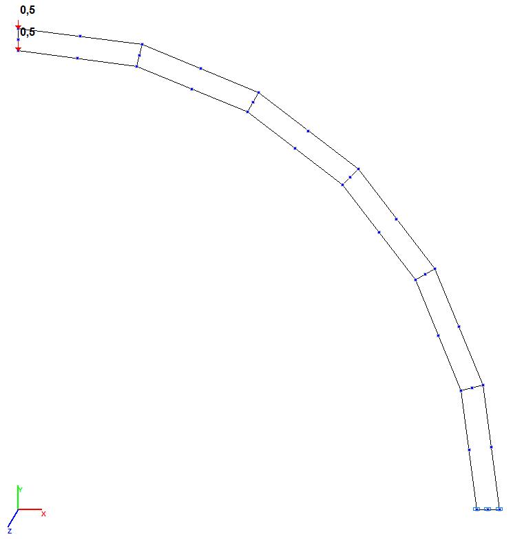
Models 7 and 8. Design model
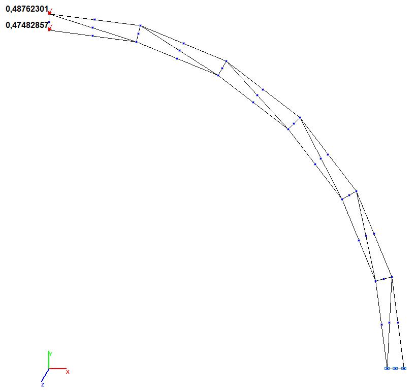
Mоdels 7 and 8. Deformed model
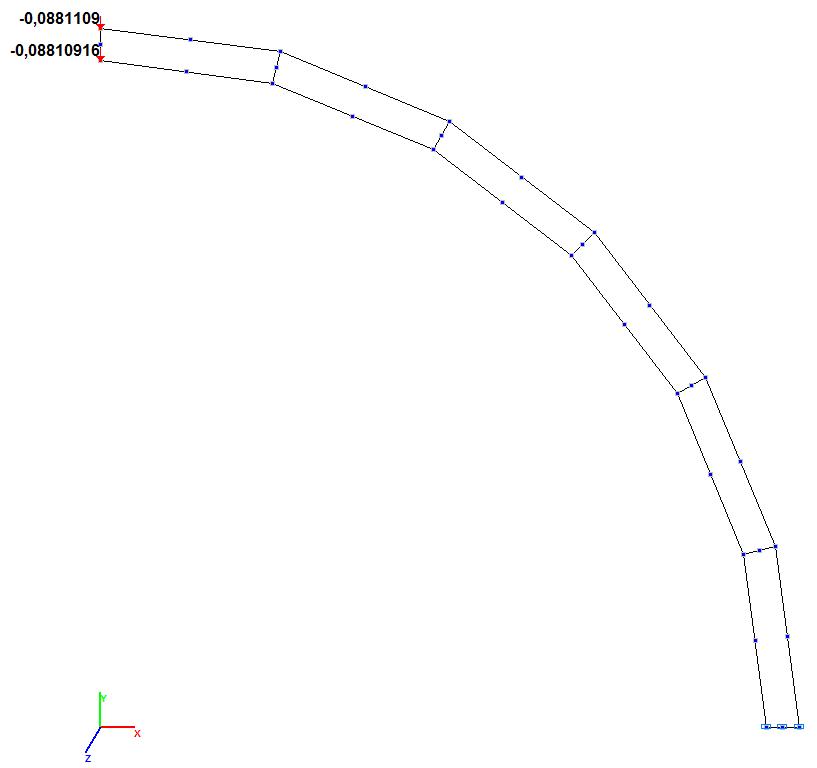
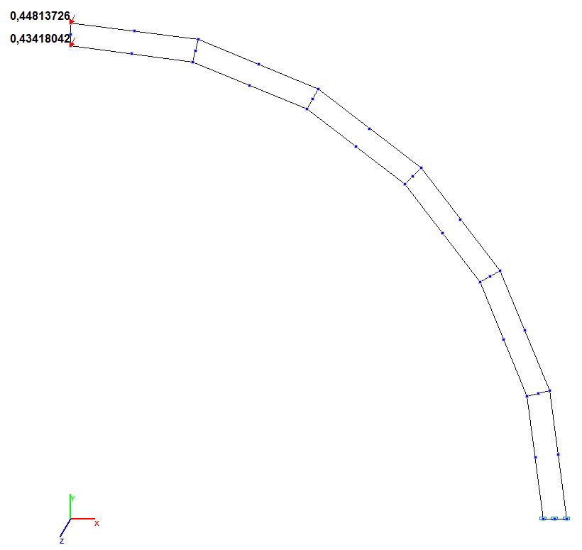
Model 7. Values of the transverse displacements Y, Z of the free end of the curvilinear cantilever beam (m, m)
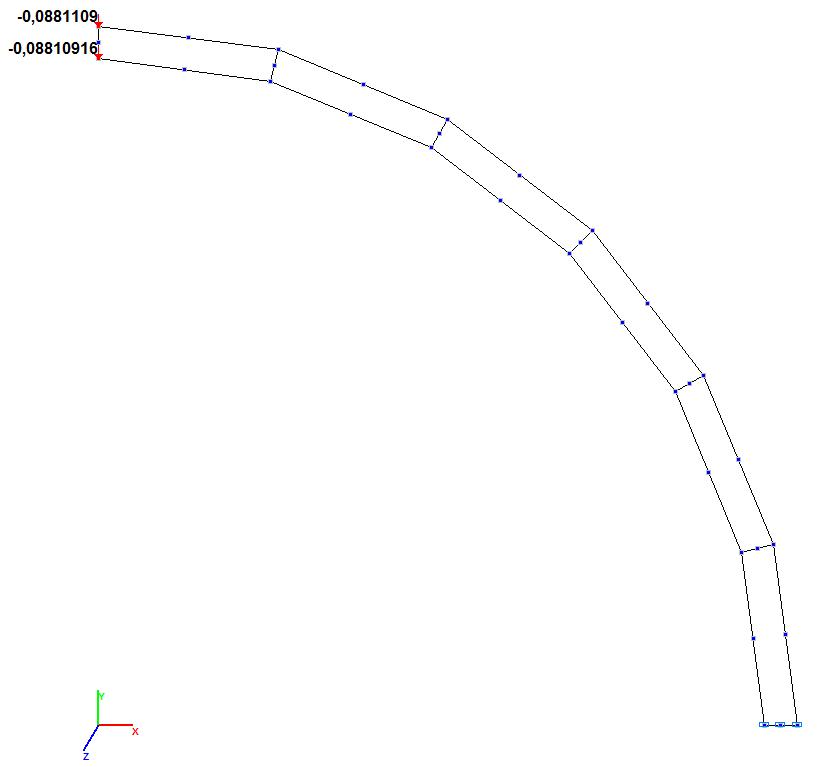
Model 8. Values of the transverse displacements Y, Z of the free end of the curvilinear cantilever beam (m, m)
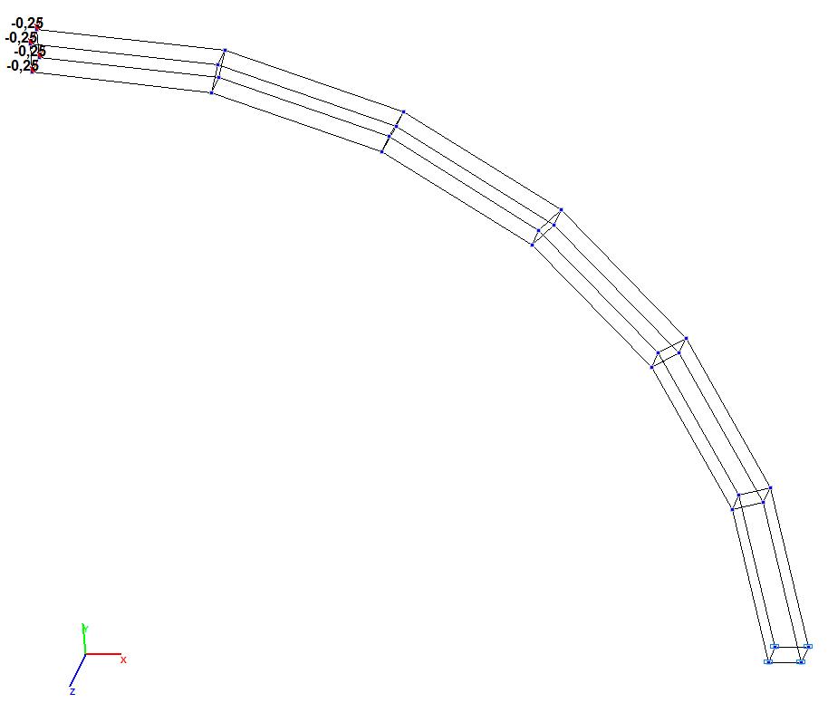
Model 9. Design model
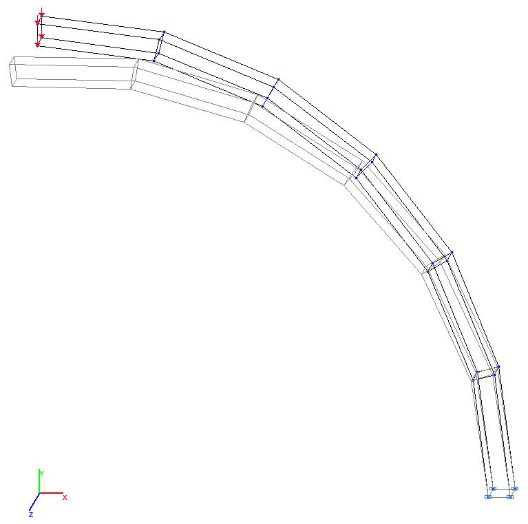
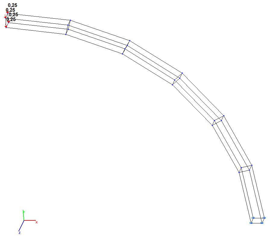
Model 9. Deformed model

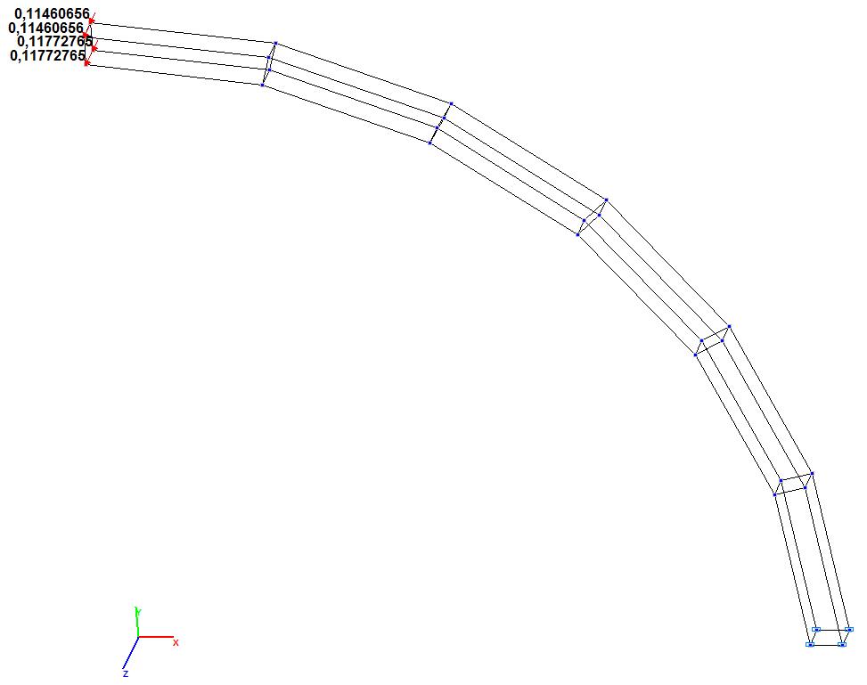
Model 9. Values of the transverse displacements Y, Z of the free end of the curvilinear cantilever beam (m, m)

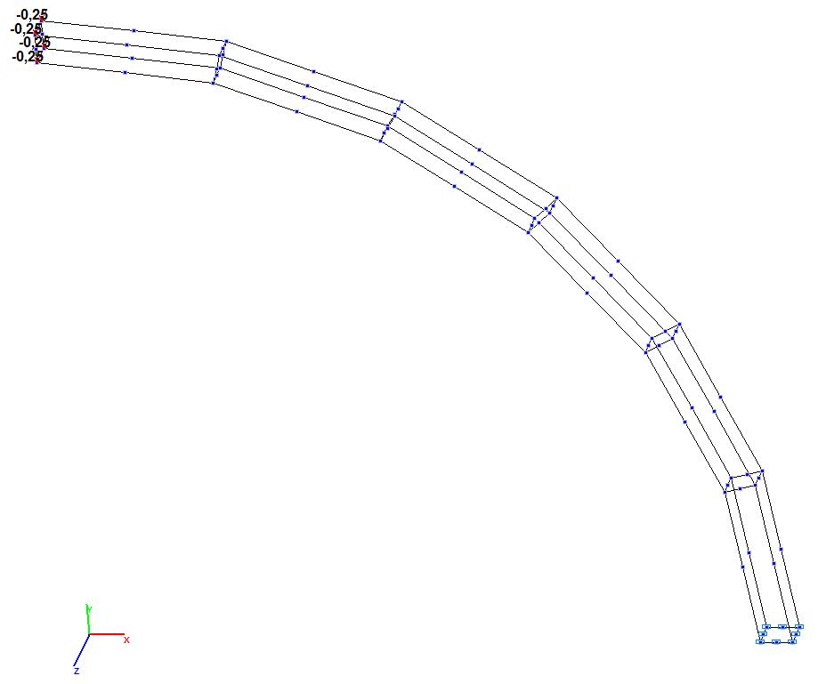
Model 10. Design model
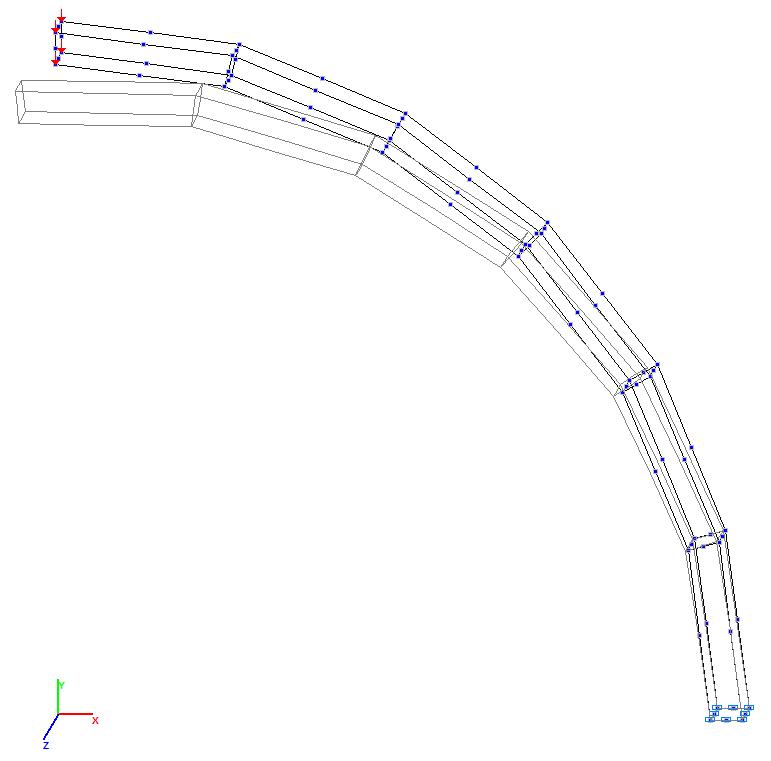
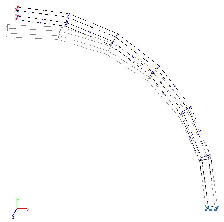
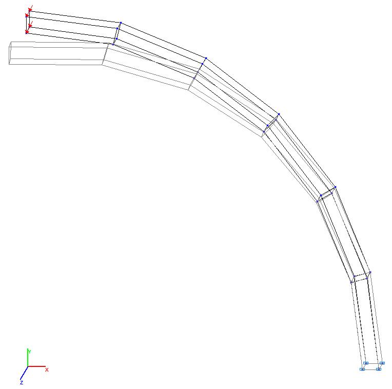
Model 10. Deformed model
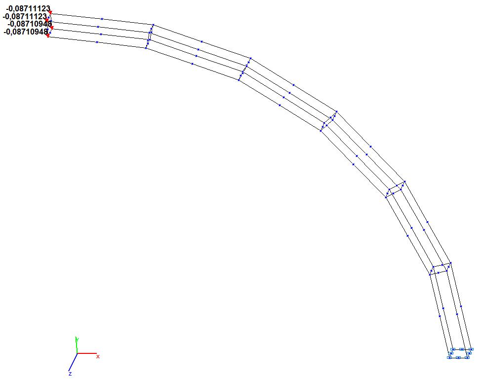

Model 10. Values of the transverse displacements Y, Z of the free end of the curvilinear cantilever beam (m, m)
Comparison of solutions:
|
Model |
Parameter |
Theory |
SCAD |
Deviation, % |
|---|---|---|---|---|
|
1 (Member type 42) |
Transverse displacement Y of the free end of the cantilever beam, m |
0.088536 |
0.002213 |
97.50 |
|
Transverse displacement Z of the free end of the cantilever beam, m |
0.454527* |
0.308152 |
32.20 |
|
|
2 (Member type 142) |
Transverse displacement Y of the free end of the cantilever beam, m |
0.088536 |
0.02213 |
97.50 |
|
Transverse displacement Z of the free end of the cantilever beam, m |
0.500466 |
0.474844 |
5.12 |
|
|
3 (Member type 44) |
Transverse displacement Y of the free end of the cantilever beam, m |
0.088536 |
0.006411 |
92.76 |
|
Transverse displacement Z of the free end of the cantilever beam, m |
0.454527* |
0.334655 |
26.37 |
|
|
4 (Member type 144) |
Transverse displacement Y of the free end of the cantilever beam, m |
0.088536 |
0.006563 |
92.59 |
|
Transverse displacement Z of the free end of the cantilever beam, m |
0.500466 |
0.487387 |
2.61 |
|
|
5 (Member type 45) |
Transverse displacement Y of the free end of the cantilever beam, m |
0.088536 |
0.088299 |
0.27 |
|
Transverse displacement Z of the free end of the cantilever beam, m |
0.454527* |
0.442069 |
2.74 |
|
|
6 (Member type 145) |
Transverse displacement Y of the free end of the cantilever beam, m |
0.088536 |
0.088299 |
0.27 |
|
Transverse displacement Z of the free end of the cantilever beam, m |
0.500466 |
0.487623 |
2.57 |
|
|
7 (Member type 50) |
Transverse displacement Y of the free end of the cantilever beam, m |
0.088536 |
0.088111 |
0.48 |
|
Transverse displacement Z of the free end of the cantilever beam, m |
0.454527* |
0.448137 |
1.41 |
|
|
8 (Member type 150) |
Transverse displacement Y of the free end of the cantilever beam, m |
0.088536 |
0.088111 |
0.48 |
|
Transverse displacement Z of the free end of the cantilever beam, m |
0.500466 |
0.490701 |
1.95 |
|
|
9 (Member type 36) |
Transverse displacement Y of the free end of the cantilever beam, m |
0.088536 |
0.006397 |
92.77 |
|
Transverse displacement Z of the free end of the cantilever beam, m |
0.500466 |
0.114607 |
77.10 |
|
|
10 (Member type 37) |
Transverse displacement Y of the free end of the cantilever beam, m |
0.088536 |
0.087111 |
1.61 |
|
Transverse displacement Z of the free end of the cantilever beam, m |
0.500466 |
0.470384 |
6.01 |
* The values of the transverse displacements Z for thin plates (not allowing for shear) are determined at the free torsional inertia moment calculated with the value of the coefficient kf, equal to 1/3 (h/b = ∞).
Notes: In the analytical solution the values of the transverse displacements Y, Z of the free end of the curvilinear cantilever beam from the respective actions are determined according to the following formulas:
\[ Y=\frac{3\cdot \pi \cdot P_{y} \cdot R^{3}}{E\cdot b\cdot h^{3}}; \quad Z=\frac{P_{z} \cdot R^{3}}{2\cdot E\cdot b^{3}\cdot h\cdot k_{f} }\cdot \left[ {6\cdot \pi \cdot k_{f} +\left( {3\cdot \pi -8} \right)\cdot \left( {1+\nu } \right)} \right], \] \[ where: \quad k_{f} =\frac{1}{3}\cdot \left\{ {1-\frac{192}{\pi^{5}}\cdot \frac{b}{h}\cdot \sum\limits_{n=1}^\infty {\left[ {\sin^{2}\left( {\frac{n\cdot \pi }{2}} \right)\cdot \frac{1}{n^{5}}\cdot th\left( {\frac{n\cdot \pi \cdot h}{2\cdot b}} \right)} \right]} } \right\}. \]