Cantilever Weightless Column with a Concentrated Mass at the Free End Subjected to a Horizontal Kinematic Displacement of a Support (Seismogram Based Analysis)

Objective: Determination of the strain state of a cantilever weightless column with a concentrated mass at the free end subjected to a horizontal kinematic displacement of a support.
Initial data file: 5.14.SPR
Seismogram file: 5.14_chart.txt
Problem formulation: The mass m is attached to the free end of the cantilever weightless column with a square cross-section. A horizontal kinematic action varying according to the harmonic law Xs = Δ·sin(θ·t) is applied to the support of the column at the initial time. Determine the natural oscillation mode and frequency ω of the cantilever column, as well as the deflection Xm of the free end of the column with the attached mass with time.
References: Kiselev V.A., Structural Mechanics. Special Course. Dynamics and Stability of Structures. Moscow, Stroyizdat, 1980, p. 65.
Initial data:
| E = 2.0·108 kN/m2 | - elastic modulus of the column material; |
| ν = 0.3 | - Poisson’s ratio; |
| b = 0.04 m | - width of the rectangular cross-section of the column; |
| h = 0.04 m | - height of the rectangular cross-section of the column; |
| L = 1.0 m | - length of the column; |
| m = 0.08 kN·s2/m | - value of the concentrated mass attached to the free end of the column; |
| Δ = 0.1 m | - amplitude value of the horizontal kinematic harmonic excitation applied to the support of the column; |
| g = 10.00 m/s2 | - gravitational acceleration; |
| I = b·h3/12 = 2.133333·10-7 m4 | - cross-sectional moment of inertia of the column. |
The following value of the frequency of the kinematic harmonic excitation θ depending on the value of the natural frequency of the column ω is considered: θ = 0.5·ω.
Finite element model: Design model – general type system, 10 bar elements of type 5. Boundary conditions are provided by imposing constraints in the node of the clamped end of the column in the directions of the degrees of freedom X, Y, Z, UX, UY, UZ. The concentrated mass is specified by transforming the static nodal load on the free end of the column m·g.
The calculation is performed in two stages: first the natural oscillation mode and natural frequency ω are determined by the modal analysis, and then the deflection Xm of the free end of the column with the attached mass with time is determined by the direct integration of the equations of motion method. The action of the kinematic harmonic excitation is described by the graph of the variation of the horizontal displacement of the support with time and is given in the form of the specified displacement of the constraint along the X axis of the global coordinate system with the scale factor of 1.0 and the delay time 0.0 s. Intervals between the time points of the displacement variation graph are equal to Δtint = Tθ, where Tθ – period of the kinematic harmonic excitation, and correspond to the integration step. When plotting the graph, the action of the specified displacement of the constraint is taken as Xs = Δ·sin(θ· n·Δtint) at the time points n·Δtint. The duration of the process is equal to t = 2·Tθ. Critical damping ratios for the 1-st and 2-nd natural frequencies are taken with the minimum value ξ = 0.0001. The conversion factor for the added static loading is equal to k = 0.981 (mass generation). Number of nodes in the design model – 11. The modal integration method is used in the calculation. The determination of the natural oscillation modes and natural frequencies is performed by the method of subspace iteration. The matrix of concentrated masses is used in the calculation.
Results in SCAD
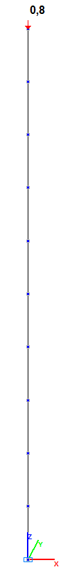
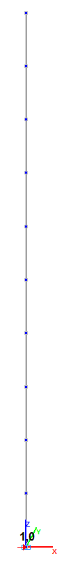
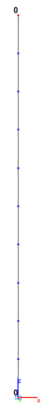
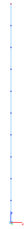
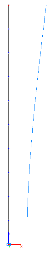
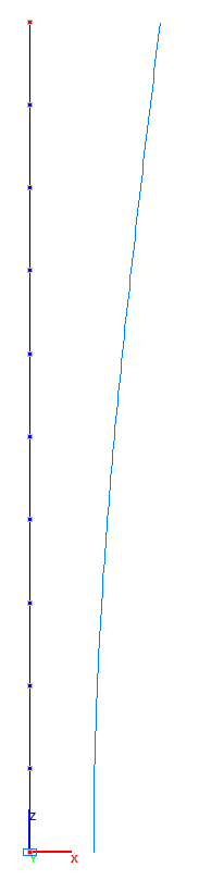
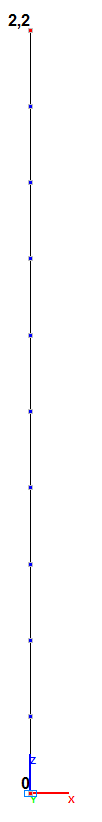
Design model and the 1-st oscillation mode
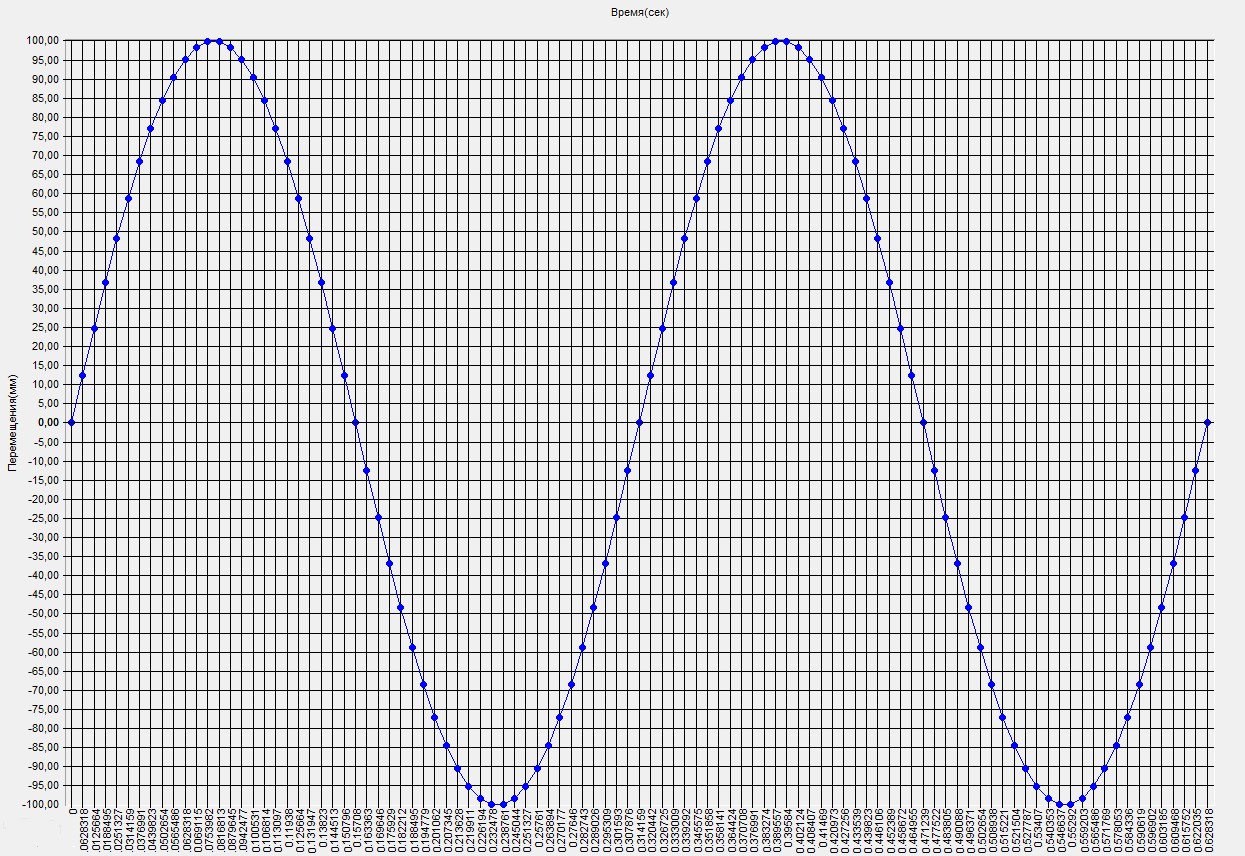
Graph of the variation of the horizontal displacement of the constraint Xs with time (mm).
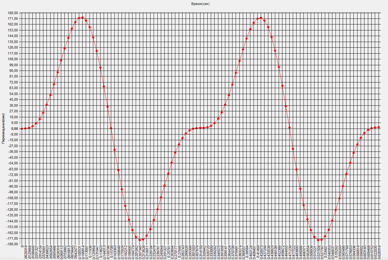
Graph of the variation of the deflection Xm of the free end of the column with the attached mass with time (mm)
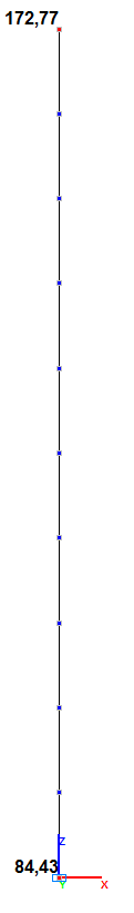
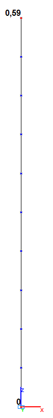

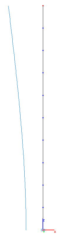
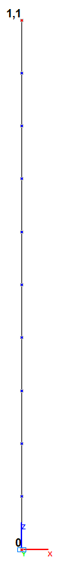
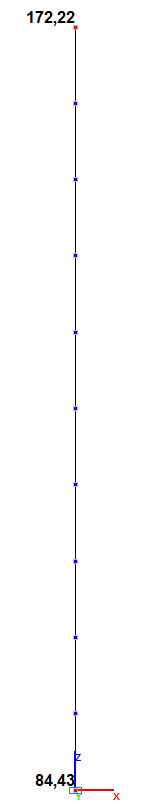
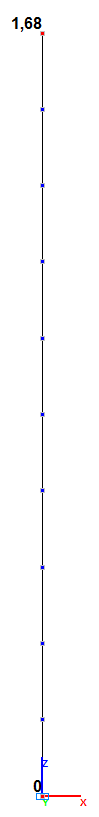
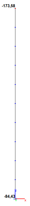
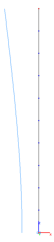
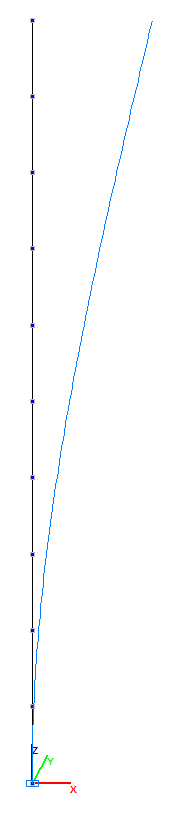
Amplitude values of the deflection Xm of the free end of the column with the attached mass and the deformed models at the respective time points (mm).
Comparison of solutions:
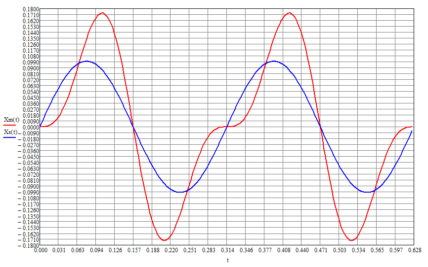
Graphs of the variation of the horizontal displacement of the constraint Xs and the deflection Xm of the free end of the column with the attached mass with time (m)
Frequency of the kinematic harmonic excitation θ = 0.5·ω
Natural frequency ω, rad/s
|
Oscillation mode |
Theory |
SCAD |
Deviations, % |
|---|---|---|---|
|
1 |
40.000 |
40.000 |
0.00 |
Amplitude values of the deflection Xm of the free end of the column with the attached mass at the frequency of the kinematic harmonic excitation θ = 0.5·ω, mm
|
Theory |
SCAD |
|||
|---|---|---|---|---|
|
Time, s |
Deflection, m |
Time, s |
Deflection, m |
Deviation, % |
|
0.000000 |
0.00 |
0.000000 |
0.00 |
— |
|
0.106814 |
172.90 |
0.106814 |
172.77 |
0.08 |
|
0.157080 |
0.00 |
0.157080 |
0.59 |
— |
|
0.207345 |
-172.90 |
0.207345 |
-173.21 |
0.18 |
|
0.314159 |
0.00 |
0.314159 |
1.10 |
— |
|
0.420973 |
172.90 |
0.420973 |
172.22 |
0.39 |
|
0.471239 |
0.00 |
0.471239 |
1.68 |
— |
|
0.521504 |
-172.90 |
0.521504 |
-173.58 |
0.39 |
|
0.628318 |
0.00 |
0.628318 |
2.20 |
— |
Notes: In the analytical solution the natural frequency ω of the cantilever column with the concentrated mass on the free end is determined according to the following formula:
\[ \omega =\sqrt {\frac{3\cdot E\cdot I}{m\cdot L^{3}}} \]
In the analytical solution the deflection Xm of the free end of the column with the attached mass with time is determined according to the following formula:
\[ X_{m} \left( t \right)=\frac{\Delta }{\left( {1-\frac{\theta^{2}}{\omega ^{2}}} \right)}\cdot \left( {\sin \left( {\theta \cdot t} \right)-\frac{\theta }{\omega }\cdot \sin \left( {\omega \cdot t} \right)} \right) \]