Non-uniform Damping
Objective: comparison of the solution of the problem (Fig. 1) by the Newmark method (SCAD) with the numerical solution obtained in MathCAD.
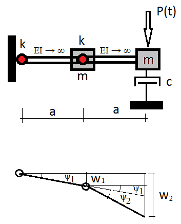
Figure 1. Two rigid weightless bodies are connected to each other and to the rigid support by springs with the stiffness k. The inertial properties of the system are represented by concentrated masses m. The local damper with the damping ratio c connects the end mass with the support.
Initial data files:
Test_local_damping.SPR - design model
TimeHist_1.txt - time function
local_damping.xmcd – MathCAD file
Finite element model: Design model – general type system, two finite elements of the elastic constraint (type 55), two finite elements of the rigid body (type 100) and one single-node damper (type 56). Number of nodes in the design model – 5. The matrix of concentrated masses is used in the calculation.
Solution description:
A deformed model is shown in Fig. 1. The following kinematic relations follow from it:
| \[ \psi_{1} =\frac{w_{1} }{a};\quad \psi_{2} =\frac{w_{2} -w_{1} }{a}-\psi _{1} =\frac{w_{2} -2w_{1} }{a} \] | (1) |
Here w1, w2 – normal deflections, and ψ1, ψ2 – deflection angles of rigid bars. The total potential energy of the system is given in the form
| \[ Э=П+W=\frac{1}{2}k\psi_{1}^{2} +\frac{1}{2}k\psi_{2}^{2} -P w_{2} \] | (2) |
where П and W – potential energy of elastic deformations and change in the potential of external forces. The kinetic energy of the system Т is given below:
| \[ T=\frac{1}{2}m\dot{{w}}_{1}^{2} +\frac{1}{2}m\dot{{w}}_{2}^{2} \] | (3) |
Applying Hamilton's variational principle
| \[ \delta \int\limits_{t1}^{t2} {Ldt=0} \] | (4) |
where L = T – Э, and adding the viscous friction forces we obtain the following equations of motion:
| \[ {\rm {\bf M\ddot{{x}}}}+{\rm {\bf C\dot{{x}}}}+{\rm {\bf Kx}}={\rm {\bf p}}\left( t \right) \] | (5) |
where
| \[ {\rm {\bf M}}=\left( {{\begin{array}{*{20}c} m & 0 \\ 0 & m \\ \end{array} }} \right),\quad {\rm {\bf C}}=\left( {{\begin{array}{*{20}c} 0 & 0 \\ 0 & c \\ \end{array} }} \right),\quad {\rm {\bf K}}=\frac{k}{a^{2}}\left( {{\begin{array}{*{20}c} 5 & {-2} \\ {-2} & 1 \\ \end{array} }} \right),\quad {\rm {\bf x}}=\left( {{\begin{array}{*{20}c} {w_{1} } \\ {w_{2} } \\ \end{array} }} \right),\quad {\rm {\bf p}}\left( t \right)=\left( {{\begin{array}{*{20}c} 0 \\ {P\left( t \right)} \\ \end{array} }} \right) \] | (6) |
The system of equations (5) is solved by MathCAD using the rkfixed procedure, which implements the fourth-order Runge-Kutta method. The function P(t) is given by the following algorithm:
 |
(7) |
The integration interval is taken as t ∈ [0, 1], a = 1 m, k = 1000 MN∙m/rad, m = 106 kg, c = 10 MN∙s/m, and the number of points approximating the unknown function is npoint = 1000. The Runge-Kutta method is an explicit integration method, therefore, it is conditionally stable. At npoint = 10 the unstable behavior of the solution is observed, the results for npoint = 100 and npoint = 1000 are slightly different at the right end of the interval, and the results for npoint = 1000 and npoint = 10000 are virtually identical. Therefore, we believe that the numerical solution for npoint = 1000 leads to virtually accurate results.
The SCAD design model is shown in Fig. 2, and the comparison of the above solution with the results obtained by the Newmark method (SCAD) is given in Fig. 4. When the Newmark method is used, the integration step is taken as Δt = 0.0001 s.
The load vs. time relationship corresponding to (7) is given in Fig. 3.
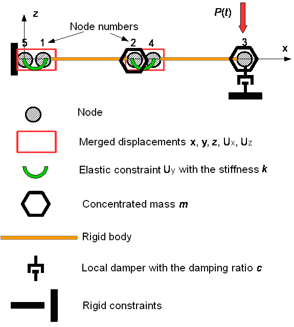
Figure 2. SCAD design model
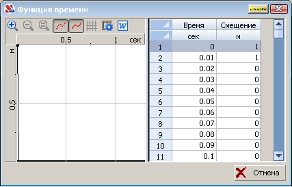
Figure 3. Load vs. time relationship
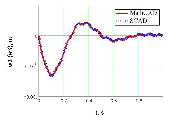
Figure 4. Vertical displacement of the cantilever end
At the time point t = 0.1 s the displacement of the cantilever end reaches a value close to the maximum (absolute value) one, and the displacement obtained by MathCAD is w2 = – 6.5393∙10–4 (Fig. 1), and the displacement obtained by the Newmark method is w3 = – 6.5170∙10–4 (Fig. 3).
Thus, the results of numerical solutions obtained by MathCAD and the Newmark method (SCAD) are virtually identical which confirms the reliability of both these methods.