Clamped Rectangular Plate of Constant Thickness Subjected to Thermal Loading
Objective: Determine the bending moments and stresses in a rectangular plate clamped on all sides at the linear temperature variation across the thickness of the plate.
Initial data file: 4_20.spr
Problem formulation: The rectangular plate of constant thickness clamped on all sides is considered. The temperature is constant in the planes parallel to the midsurface and varies linearly across the thickness of the plate. Determine: the displacement w, bending moments Mx, My and maximum thermal stress σ.
References: S. Timoshenko, S. Woinowsky-Krieger, Theory of Plates and Shells. — M.:Nauka, 1963.
Initial data:
| E = 2.0·108 kPa | - elastic modulus, |
| μ = 0.3 | - Poisson’s ratio, |
| aх = 1.5 m | - width of the plate, |
| aу = 2.5 m | - length of the plate |
| h = 0.02 m | - thickness of the plate, |
| α= 1.5·10-5 1/С0 | - linear thermal expansion coefficient of the material, |
| ΔТ = 20 С0 | - temperature difference between the upper and lower surfaces of the plate |
Constraints: rigid restraint of nodes along the contour (displacement u=v=w = θx = θy= θz = 0)
Finite element model: Design model – general type system. Plate elements – 200 four-node elements of type 41. Number of nodes in the design model – 231.
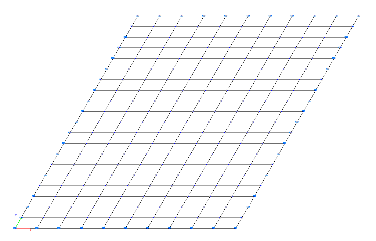
Design model
Results in SCAD
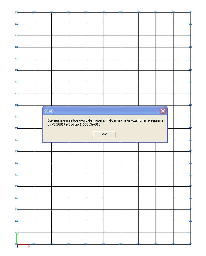
Values of displacements w (mm)
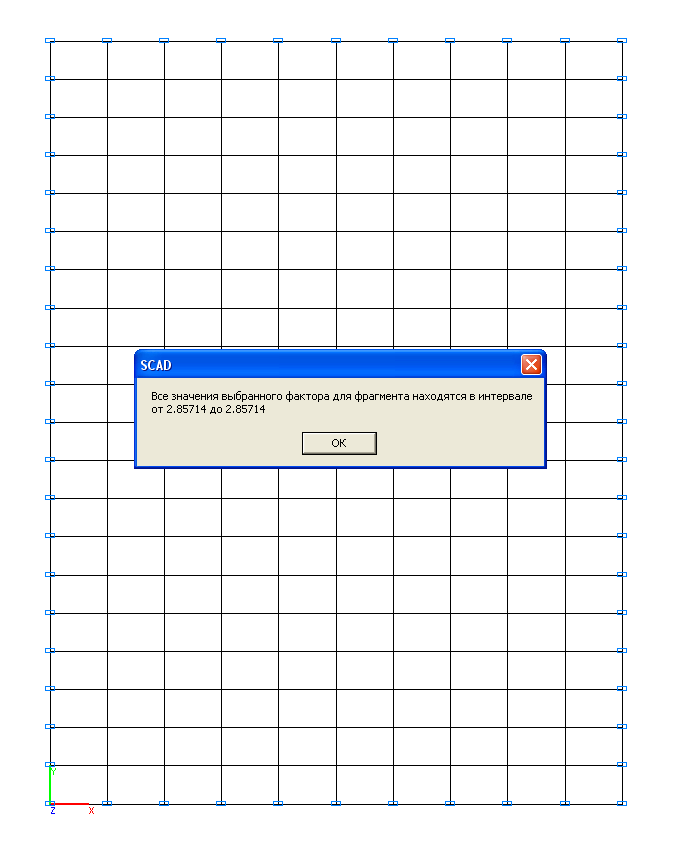
Values of bending moments Mx (kN·m/m)
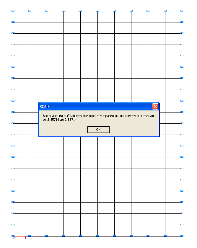
Values of bending moments My (kN·m/m)
Values of stresses on the upper surface of the plate σ (kN/m2)
Comparison of solutions:
|
Parameter |
Theory |
SCAD |
Deviations, % |
|---|---|---|---|
|
Displacement w, mm |
0.00 |
0.00 |
─ |
|
Bending moments Мх = Му , kN∙m /m |
2.857 |
2.857 |
0.00 |
|
Maximum thermal stress, kPa |
42857 |
42857 |
0.00 |
Notes: In the analytical solution the bending moments Mx, My and maximum thermal stress σ in the clamped plate subjected to the linear temperature variation across the thickness of the plate can be determined according to the following formulas (S. Timoshenko, S. Woinowsky-Krieger, Theory of Plates and Shells. — M.:Nauka, 1963, p. 64):
\[M_{x} =M_{y} =D\cdot \frac{\alpha \cdot \Delta T\cdot \left( {1+\mu } \right)}{h}, where: \] \[ D=\frac{E\cdot h^{3}}{12\cdot \left( {1-\mu^{2}} \right)}, \] \[ \sigma =\frac{\alpha \cdot \Delta T\cdot E}{2\cdot \left( {1-\mu } \right)}. \]