Cylindrical Vertical Tank with a Wall of Constant Thickness with a Flat Bottom Subjected to Internal Fluid Pressure

Objective: Determination of the stress-strain state of a cylindrical vertical tank with a wall of constant thickness clamped in a flat bottom subjected to internal fluid pressure which varies linearly with height.
Initial data file: 4_32.spr
Problem formulation: The cylindrical vertical tank with a wall of constant thickness is clamped in a flat bottom and subjected to internal pressure of the liquid with the specific weight γ. Determine the bending moments and longitudinal forces acting on the midsurface of the tank wall in the meridian Mx, Nx and in the circumferential Mφ, Nφ directions, as well as the radial displacements w of the tank wall.
References: S.P. Timoshenko, Theory of Plates and Shells. — Moscow: OGIZ. Gostekhizdat, 1948.
Initial data:
| E = 2.1·108 kPa | - elastic modulus; |
| ν = 0.3 | - Poisson’s ratio; |
| h = 0.01 m | - thickness of the tank wall; |
| a = 5.0 m | - radius of the midsurface of the tank wall; |
| d = 5.0 m | - height of the tank; |
| γ = 10.0 kN/m3 | - specific weight of the liquid in the tank. |
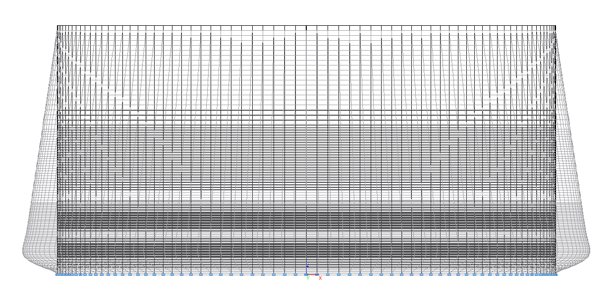
Finite element model: Design model – general type system, shell elements – 15840 four-node elements of type 44. The spacing of the finite element mesh in the meridian direction is 0.025 m at the height x from the bottom from 0.0 m to 1.5 m; 0.050 m at the height x from the bottom from 1.5 m to 3.0 m; 0.100 m at the height x from the bottom from 3.0 m to 5.0 m; and in the circumferential direction the spacing is 2.5º. The boundary conditions at the clamping into the bottom are provided by imposing constraints in all directions of the angular and linear displacements. Number of nodes in the design model – 15984.
Results in SCAD
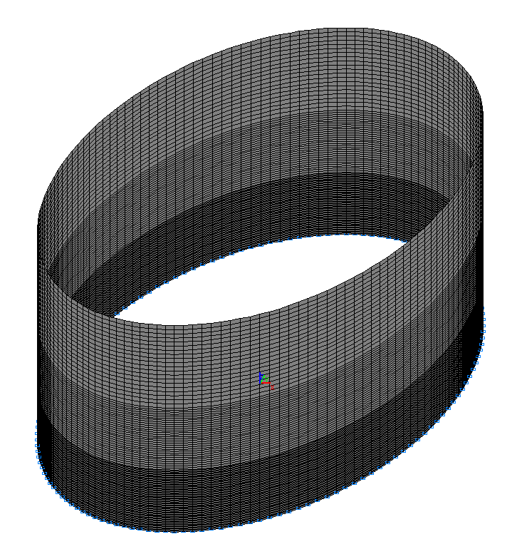
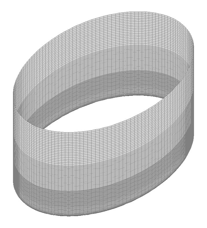
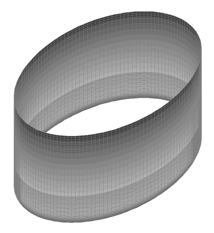
Design model
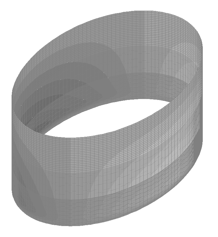
Deformed model
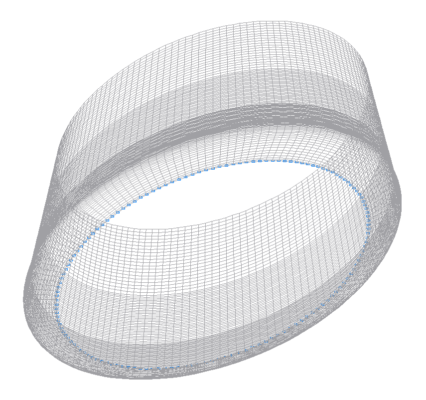
Deformed model
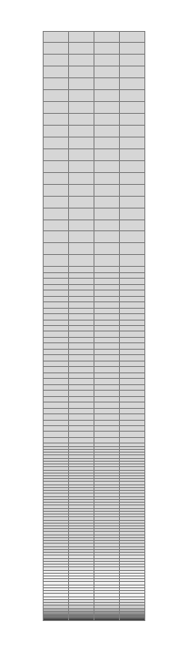
Values of radial displacements w (mm)
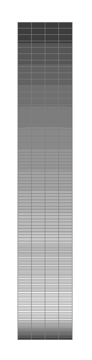
Values of radial displacements w (mm) for the fragment of the model from the section with the central angle of 10.0º
Values of bending moments acting on the midsurface of the tank wall in the meridian direction Mx (kN∙m/m)
Values of bending moments acting on the midsurface of the tank wall in the meridian direction Mx (kN∙m/m) for the fragment of the model from the section with the central angle of 10.0º
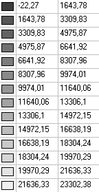
Values of longitudinal forces acting on the midsurface of the tank wall in the circumferential direction Nφ (kN/m2)
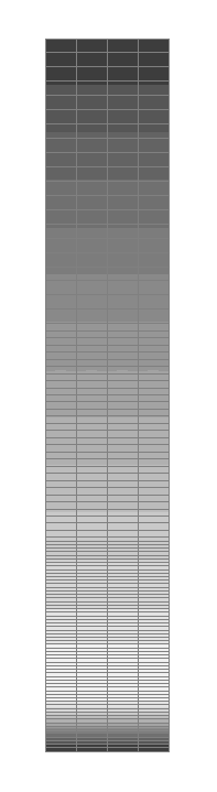
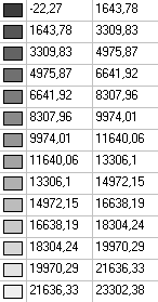
Values of longitudinal forces acting on the midsurface of the tank wall in the circumferential direction Nφ (kN/m2) for the fragment of the model from the section with the central angle of 10.0º
Comparison of solutions:
|
x, m |
w, mm |
Mx, kN∙m/m |
Nφ, kN/m |
||||||
|---|---|---|---|---|---|---|---|---|---|
|
Theory |
SCAD |
Deviations, % |
Theory |
SCAD |
Deviations, % |
Theory |
SCAD |
Deviations, % |
|
|
0.000 |
0.000 |
0.000 |
─ |
-0.7302 |
-0.7267 |
0.48 |
0.00 |
-22.27∙0.01 = -0.22 |
─ |
|
0.025 |
0.011 |
0.011 |
0.00 |
-0.5321 |
-0.5253 |
1.28 |
4.52 |
432.34∙0.01 = 4.32 |
4.42 |
|
0.050 |
0.039 |
0.039 |
0.00 |
-0.3644 |
-0.3564 |
2.20 |
16.33 |
1612.89∙0.01 = 16.13 |
1.22 |
|
0.075 |
0.079 |
0.078 |
1.27 |
-0.2256 |
-0.2179 |
3.41 |
33.15 |
3285.96∙0.01 = 32.86 |
0.87 |
|
0.100 |
0.126 |
0.125 |
0.79 |
-0.1134 |
-0.1069 |
5.73 |
53.08 |
5261.88∙0.01 = 52.62 |
0.87 |
|
0.125 |
0.178 |
0.176 |
1.12 |
-0.0252 |
-0.0204 |
─ |
74.59 |
7388.51∙0.01 = 73.89 |
0.94 |
|
0.150 |
0.230 |
0.227 |
1.30 |
0.0419 |
0.0448 |
─ |
96.46 |
9547.11∙0.01 = 95.47 |
1.03 |
|
0.175 |
0.280 |
0.277 |
1.07 |
0.0907 |
0.0918 |
1.21 |
117.78 |
11648.07∙0.01 = 116.48 |
1.10 |
|
0.200 |
0.328 |
0.324 |
1.22 |
0.1241 |
0.1235 |
0.48 |
137.88 |
13626.65∙0.01 = 136.27 |
1.17 |
|
0.225 |
0.372 |
0.367 |
1.34 |
0.1448 |
0.1428 |
1.38 |
156.30 |
15439.08∙0.01 = 154.39 |
1.22 |
|
0.250 |
0.411 |
0.406 |
1.22 |
0.1550 |
0.1520 |
1.94 |
172.76 |
17058.39∙0.01 = 170.58 |
1.26 |
|
0.275 |
0.445 |
0.440 |
1.12 |
0.1572 |
0.1535 |
2.35 |
187.11 |
18471.73∙0.01 = 184.72 |
1.28 |
|
0.300 |
0.475 |
0.468 |
1.47 |
0.1532 |
0.1491 |
2.68 |
199.32 |
19676.68∙0.01 = 196.77 |
1.28 |
|
0.325 |
0.499 |
0.492 |
1.40 |
0.1447 |
0.1405 |
2.90 |
209.44 |
20678.89∙0.01 = 206.79 |
1.27 |
|
0.350 |
0.518 |
0.512 |
1.16 |
0.1332 |
0.1291 |
3.08 |
217.60 |
21489.82∙0.01 = 214.90 |
1.24 |
|
0.375 |
0.533 |
0.527 |
1.13 |
0.1198 |
0.1160 |
3.17 |
223.93 |
22124.83∙0.01 = 221.25 |
1.20 |
|
0.400 |
0.544 |
0.538 |
1.10 |
0.1054 |
0.1021 |
3.13 |
228.64 |
22601.65∙0.01 = 226.02 |
1.15 |
|
0.425 |
0.552 |
0.546 |
1.09 |
0.0909 |
0.0881 |
3.08 |
231.90 |
22939.13∙0.01 = 229.39 |
1.08 |
|
0.450 |
0.557 |
0.551 |
1.08 |
0.0767 |
0.0745 |
2.87 |
233.93 |
23156.28∙0.01 = 231.56 |
1.01 |
|
0.475 |
0.559 |
0.554 |
0.89 |
0.0633 |
0.0617 |
2.53 |
234.90 |
23271.56∙0.01 = 232.72 |
0.93 |
|
0.500 |
0.560 |
0.555 |
0.89 |
0.0510 |
0.0500 |
1.96 |
235.01 |
23302.38∙0.01 = 233.02 |
0.85 |
|
0.550 |
0.555 |
0.552 |
0.54 |
0.0303 |
0.0302 |
0.33 |
233.29 |
23172.87∙0.01 = 231.73 |
0.67 |
|
0.600 |
0.547 |
0.545 |
0.37 |
0.0148 |
0.0155 |
4.73 |
229.89 |
22875.52∙0.01 = 228.76 |
0.49 |
|
0.650 |
0.537 |
0.535 |
0.37 |
0.0043 |
0.0055 |
─ |
225.66 |
22490.85∙0.01 = 224.91 |
0.33 |
|
0.700 |
0.527 |
0.526 |
0.19 |
-0.0022 |
-0.0008 |
─ |
221.17 |
22074.31∙0.01 = 220.74 |
0.19 |
|
0.750 |
0.516 |
0.516 |
0.00 |
-0.0055 |
-0.0042 |
─ |
216.79 |
21660.60∙0.01 = 216.61 |
0.08 |
|
0.800 |
0.506 |
0.506 |
0.00 |
-0.0067 |
-0.0055 |
─ |
212.70 |
21268.60∙0.01 = 212.69 |
0.00 |
|
0.850 |
0.498 |
0.498 |
0.00 |
-0.0066 |
-0.0056 |
─ |
208.97 |
20906.05∙0.01 = 209.06 |
0.04 |
|
0.900 |
0.490 |
0.490 |
0.00 |
-0.0057 |
-0.0049 |
─ |
205.59 |
20573.53∙0.01 = 205.74 |
0.07 |
|
0.950 |
0.482 |
0.483 |
0.21 |
-0.0045 |
-0.0039 |
─ |
202.53 |
20267.56∙0.01 = 202.68 |
0.07 |
|
1.000 |
0.475 |
0.476 |
0.21 |
-0.0032 |
-0.0028 |
─ |
199.71 |
19982.79∙0.01 = 199.83 |
0.06 |
Notes: In the analytical solution the bending moments and longitudinal forces acting on the midsurface of the tank wall in the meridian Mx, Nx and circumferential Mφ, Nφ directions, as well as the radial displacements w of the tank wall can be determined according to the following formulas (S.P. Timoshenko, Theory of Plates and Shells. — Moscow: OGIZ. Gostekhizdat, 1948, p. 388):
\[ w=\frac{\gamma \cdot a^{2}\cdot d}{E\cdot h}\cdot \left( {1-\frac{x}{d}-e^{-\beta \cdot x}\cdot \left( {\cos \left( {\beta \cdot x} \right)+\left( {1-\frac{1}{\beta \cdot d}} \right)\cdot \sin \left( {\beta \cdot x} \right)} \right)} \right); \] \[ M_{x} =\frac{\gamma \cdot a\cdot d\cdot h}{\sqrt {12\cdot \left( {1-\nu ^{2}} \right)} }\cdot e^{-\beta \cdot x}\cdot \left( {\sin \left( {\beta \cdot x} \right)-\left( {1-\frac{1}{\beta \cdot d}} \right)\cdot \cos \left( {\beta \cdot x} \right)} \right); \] \[ M_{\phi } =\nu \cdot M_{x} =\frac{\gamma \cdot a\cdot d\cdot h\cdot \nu }{\sqrt {12\cdot \left( {1-\nu^{2}} \right)} }\cdot e^{-\beta \cdot x}\cdot \left( {\sin \left( {\beta \cdot x} \right)-\left( {1-\frac{1}{\beta \cdot d}} \right)\cdot \cos \left( {\beta \cdot x} \right)} \right); \] \[ N_{x} =0; \quad N_{\phi } =\frac{E\cdot h}{a}\cdot w=\gamma \cdot a\cdot d\cdot \left( {1-\frac{x}{d}-e^{-\beta \cdot x}\cdot \left( {\cos \left( {\beta \cdot x} \right)+\left( {1-\frac{1}{\beta \cdot d}} \right)\cdot \sin \left( {\beta \cdot x} \right)} \right)} \right),\quad where: \]\[ \beta =\sqrt[4]{\frac{3\cdot \left( {1-\nu^{2}} \right)}{a^{2}\cdot h^{2}}}. \]