Plane Truss Subjected to Instantaneous Pulses Concentrated in Non-Supporting Nodes of the Bottom Chord
Objective: Determination of the strain state of a plane truss subjected to instantaneous pulses concentrated in non-supporting nodes of the bottom chord.
Initial data files: 5.11.spr, График_5.11.txt
Problem formulation: The plane two-span truss with parallel chords and a diagonal lattice with three panels of equal length in each span is supported by the bottom chord. Masses M are concentrated and concentrated instantaneous transverse pulses S are applied in the intermediate (non-supporting) nodes of the bottom chord. Determine the natural oscillation modes and natural frequencies ω of the plane truss, as well as the transverse displacements of the nodal masses Z with time.
References: Rabinovich I.M., Sinitsyn A.P., Luzhin O.V., Terenin V.M., Analysis of Structures Subject to Pulse Actions, Moscow, Stroyizdat, 1970, p. 153.
Initial data:
| E = 2.0·108 tf/m2 | - elastic modulus; |
| F = 1·10-2 m2 | - cross-sectional area of the truss elements except for the column above the middle support; |
| 2· F = 2·10-2 m2 | - cross-sectional area of the column above the middle support; |
| a = 2.0 m | - height of the truss and length of the truss panel; |
| M = 16.0 tf·s2/m | - value of the concentrated masses in the intermediate (non-supporting) nodes of the truss bottom chord; |
| S = 4.0· tf∙s | - value of the concentrated instantaneous transverse pulses applied in the intermediate (non-supporting) nodes of the truss bottom chord; |
| g = 10.00 m/s2 | - gravitational acceleration. |
Finite element model: Since the structure and the applied loads are symmetric, only a half of the truss is considered with the restraints of the bottom and top chords on the symmetry axis in the longitudinal (horizontal) direction (degree of freedom X) and halving the stiffness of the column above the middle support. Design model – plane hinged bar system, 11 bar elements of type 1. Boundary conditions of the support nodes of the truss bottom chord are provided by imposing constraints in the direction of the degree of freedom Z. The concentrated masses are specified by transforming the static nodal loads M·g.
The calculation is performed in two stages: first the natural oscillation modes and natural frequencies ω are determined by the modal analysis, and then the transverse displacements of the nodal masses Z with time are determined by the direct integration of the equations of motion method. The action of the concentrated instantaneous transverse pulses is described by the graph of the load variation with time and is given in the form of nodal forces acting along the Z axis of the global coordinate system with the scale factor of 1.0 and the delay time 0.0 s. Intervals between the time points of the load variation graph are equal to Δtint = 0.00001 s and correspond to the integration step. When plotting the graph the pulse action is taken with a linear shape function, force value P = 400000 tf and duration Δtint = 0.00001 s. The duration of the process is equal to t = 0.12 s, which roughly corresponds to twice the value of the fundamental period of oscillations 4·π/ω1. Critical damping ratios for the 1-st and 2-nd natural frequencies are taken with the minimum value ξ = 0.0001. The conversion factor for the added static loading is equal to k = 0.981 (mass generation). Number of nodes in the design model – 7. The determination of the natural oscillation modes and natural frequencies is performed by the method of subspace iteration. The matrix of concentrated masses is used in the calculation.
Results in SCAD

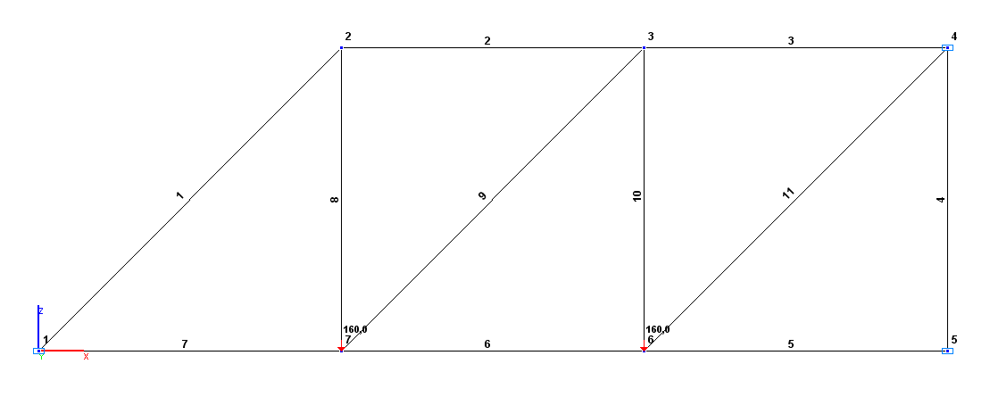
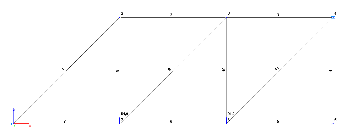
Design model
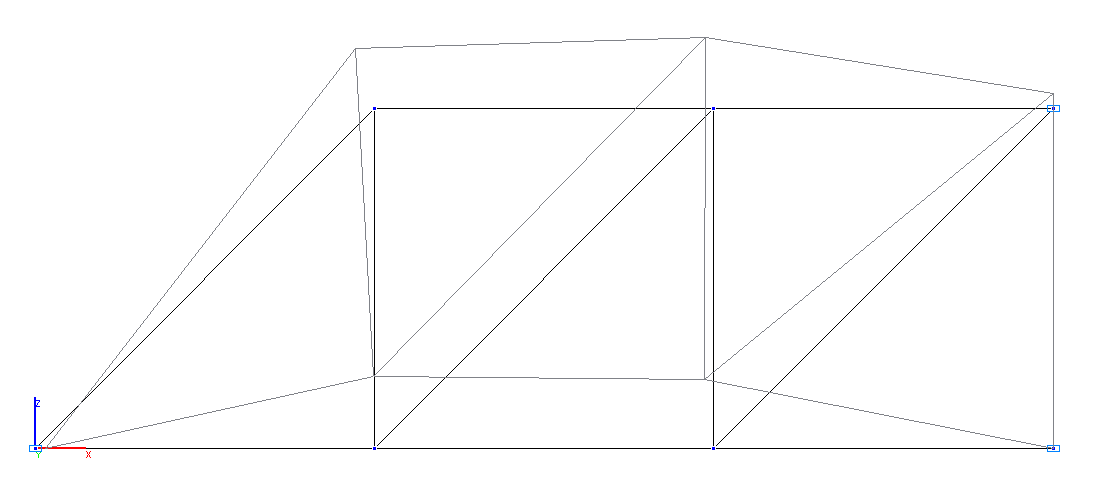
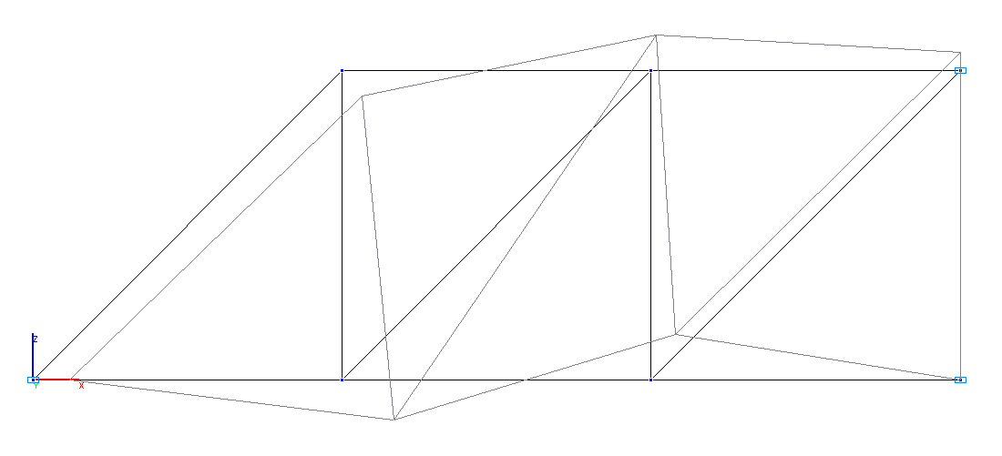
1-st and 2-nd natural oscillation modes (symmetric)
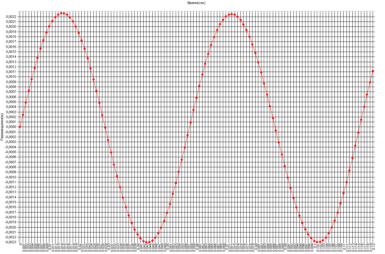
Graph of the variation of the transverse displacements of the nodal mass Z7 (closest to the end support) with time (m)

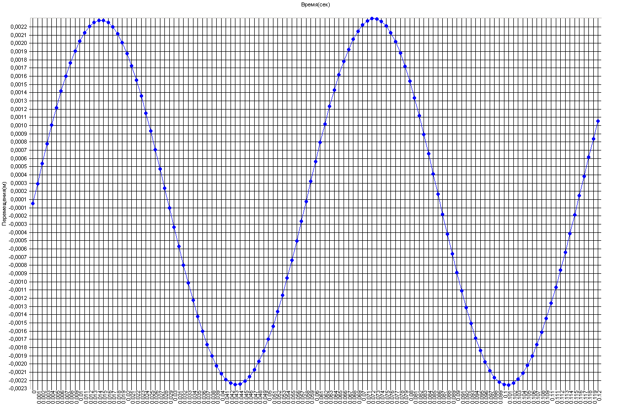
Graph of the variation of the transverse displacements of the nodal mass Z6 (closest to the middle support) with time (m)
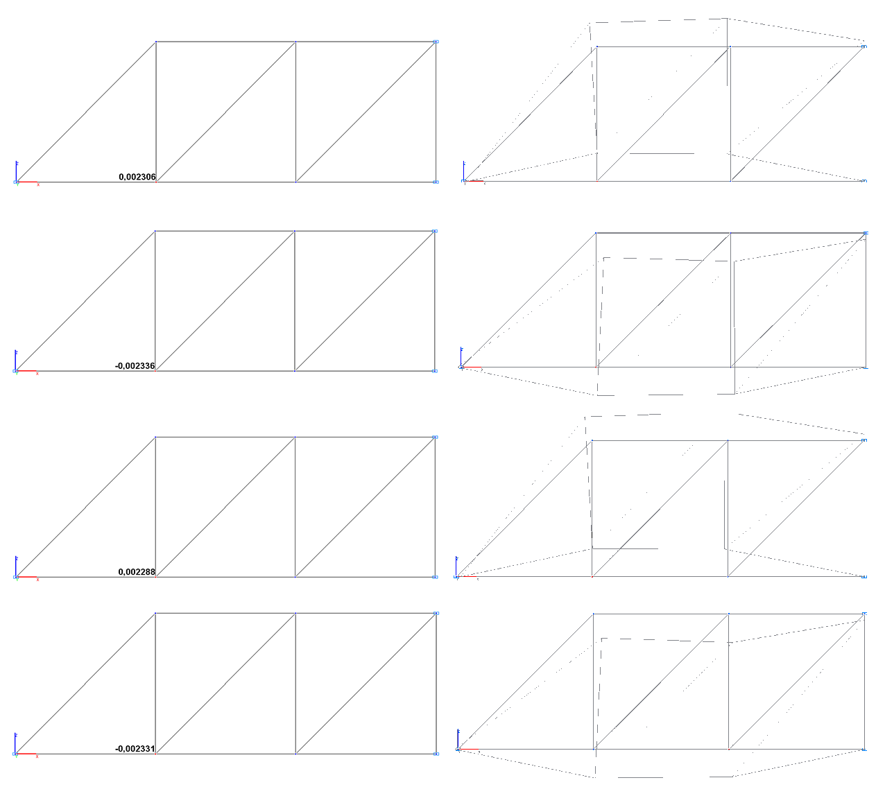
Amplitude values of the transverse displacements of the nodal mass Z7 (m) and the deformed models at the respective time points

Amplitude values of the transverse displacements of the nodal mass Z6 (m) and the deformed models at the respective time points
Comparison of solutions:
Natural frequencies ω, rad/s
|
Oscillation mode |
Theory |
SCAD |
Deviations, % |
|---|---|---|---|
|
1 |
112.0 |
108.8 |
2.86 |
|
2 |
208.0 |
197.4 |
5.10 |
Amplitude values of the transverse displacements of the nodal masses Z
|
Nodal mass |
Theory |
SCAD |
|||
|---|---|---|---|---|---|
|
Time, s |
Displacement, m |
Time, s |
Displacement, m |
Deviations, % |
|
|
7 |
0.0142 |
0.002264 |
0.0144 |
0.002306 |
1.86 |
|
7 |
0.0420 |
-0.002280 |
0.0433 |
-0.002336 |
2.46 |
|
7 |
0.0702 |
0.002251 |
0.0720 |
0.002288 |
1.64 |
|
7 |
0.0982 |
-0.002287 |
0.1014 |
-0.002331 |
1.92 |
|
6 |
0.0139 |
0.002209 |
0.0145 |
0.002249 |
1.81 |
|
6 |
0.0422 |
-0.002192 |
0.0432 |
-0.002214 |
1.00 |
|
6 |
0.0701 |
0.002222 |
0.0724 |
0.002267 |
2.03 |
|
6 |
0.0982 |
-0.002185 |
0.1006 |
-0.002220 |
1.60 |
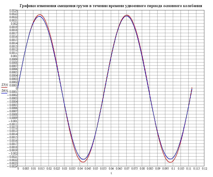
 Graphs of the variation of the transverse displacements of the nodal masses Z7 and Z6 with time according to the theoretical solution (m)
Notes: In addition to taking the symmetry into account the following assumptions were made when deriving the analytical solution:
- the displacement of masses in the longitudinal (horizontal) direction is neglected;
- the difference between the mutual transverse (vertical) displacements of the lower and upper nodes of each vertical of the truss is neglected, and the masses are concentrated only in the lower nodes.
In the analytical solution the natural frequencies of oscillations ω of the plane truss are determined according to the following formulas:
\[ \omega_{7} =0.448\cdot \sqrt {\frac{E\cdot F}{a\cdot M}} ; \quad \omega_{6} =0.832\cdot \sqrt {\frac{E\cdot F}{a\cdot M}} . \]
In the analytical solution the transverse displacements of the nodal masses of the plane truss Z with time are determined according to the following formulas:
\[ Z_{7} =1\cdot \frac{1.016\cdot S}{0.448\cdot M}\cdot \sqrt {\frac{a\cdot M}{E\cdot F}} \cdot \sin \left( {\omega_{1} \cdot t} \right)-1\cdot \frac{0.016\cdot S}{0.832\cdot M}\cdot \sqrt {\frac{a\cdot M}{E\cdot F}} \cdot \sin \left( {\omega_{2} \cdot t} \right); \] \[ Z_{6} =0.972\cdot \frac{1.016\cdot S}{0.448\cdot M}\cdot \sqrt {\frac{a\cdot M}{E\cdot F}} \cdot \sin \left( {\omega_{1} \cdot t} \right)+1.028\cdot \frac{0.016\cdot S}{0.832\cdot M}\cdot \sqrt {\frac{a\cdot M}{E\cdot F}} \cdot \sin \left( {\omega_{2} \cdot t} \right). \]
The deviations from the theory for the natural frequencies of oscillations are due to the fact that the “manual” calculation in the source is performed with significant errors.