Natural Oscillations of a Spatial Pipeline Clamped at the Edges (Hougaard’s Problem)

Objective: Modal analysis of a spatial pipeline clamped at the edges.
Initial data file: 5_1.spr
Problem formulation: Determine the natural oscillation modes and natural frequencies f of the spatial steel pipeline composed of three mutually orthogonal straight segments connected in series by fittings, clamped at the edges and filled with water.
References: William Hovgaard, Stresses in Three-dimensional Pipe Bends. Transactions of ASME, vol. 57, FSP 75-12, 1935.
Initial data:
| E = 24.0·106 psi = 1.654740·108 kPa | - elastic modulus; |
| ν = 0.3 | - Poisson’s ratio; |
| De = 7.288 in = 0.185115 m | - outer diameter of the pipe cross-section; |
| t = 0.241 in = 0.006121 m | - thickness of the pipe cross-section; |
| ρs = 0.283 lb/in3 = 7.833 t/m3 | - density of the pipe material (steel); |
| ρw = 0.036 lb/in3 = 0.996 t/m3 | - density of the filling material (water); |
| Lstr1 = 108.9 in = 2.766 m | - length of the first straight section of the pipeline; |
| Lstr2 = 35.6 in = 0.904 m | - length of the second straight section of the pipeline; |
| Lstr3 = 41.0 in = 1.041 m | - length of the third straight section of the pipeline; |
| Relb = 36.3 in = 0.922 m | - radius of the axis of the pipeline fittings; |
stiffness properties and masses:
| EA = E·(π·De2/4)·(1-(1-2·t/De)2) = 569598 kN | - axial stiffness of the pipe cross-section; |
| EIb,str = E·(π·De4/64)·(1-(1-2·t/De)4) = 2283.81 kN·m | - bending stiffness of the cross-section of the straight segment of the pipe; |
| EIb,elb = E·(π·De4/64)·(1-(1-2·t/De)4)/k = 995.824 kN·m | - bending stiffness of the cross-section of the pipe fitting (taking into account the flattening), |
| where: | |
| k = (10+12·λ2)/ (1+12·λ2) = 2.293391 | - Von Karman coefficient of flexibility, |
| λ = t·Relb/((De-2·t)/4) = 0.704654 | - geometric parameter; |
| GIt = (E/(2·(1+ ν)) ·(π·De4/32)·(1-(1-2·t/De)4) = 1756.78 kN∙m | - torsional stiffness of the pipe cross-section; |
| m = ·(π·De2/4)·(ρs -( ρs- ρw)(1-2·t/De)2)·g = 0.4938 kN∙m | - linear static load from the weight of the pipe filled with water. |
Finite element model: Design model – general type system, pipeline elements – 38 bar elements of type 5. The spacing of the finite element mesh in the longitudinal direction (along the X1 axis of the local coordinate system) is ≈ 0.2 m. Boundary conditions are provided by imposing constraints in the directions of the degrees of freedom X, Y, Z, UX, UY, UZ for the end nodes of the pipeline. The distributed mass is specified by transforming the static load from the weight of the pipe filled with water, m. Number of nodes in the design model – 39. The determination of the natural oscillation modes and natural frequencies is performed by the method of subspace iteration. The matrix of concentrated masses is used in the calculation.
Results in SCAD


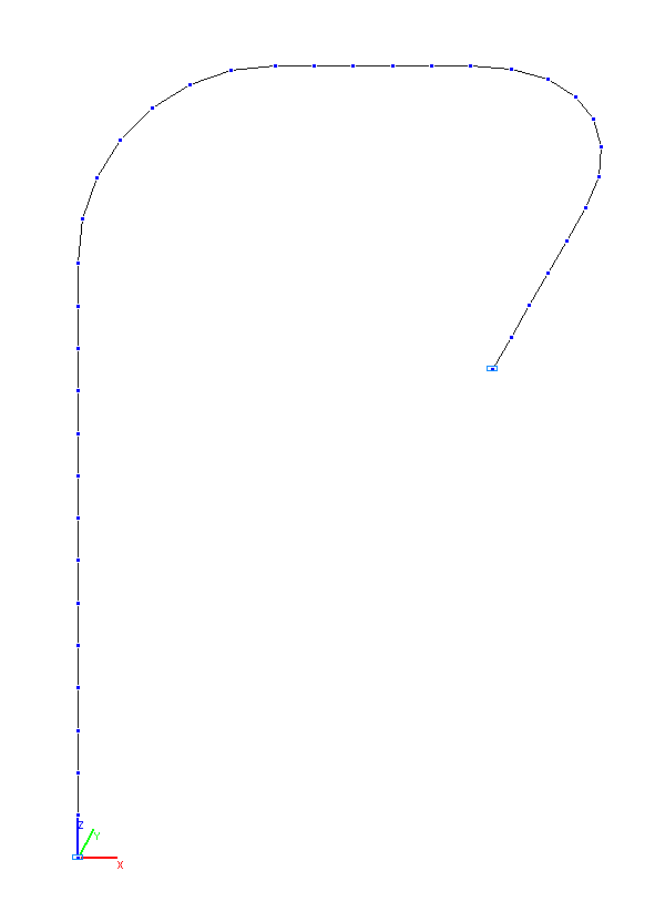
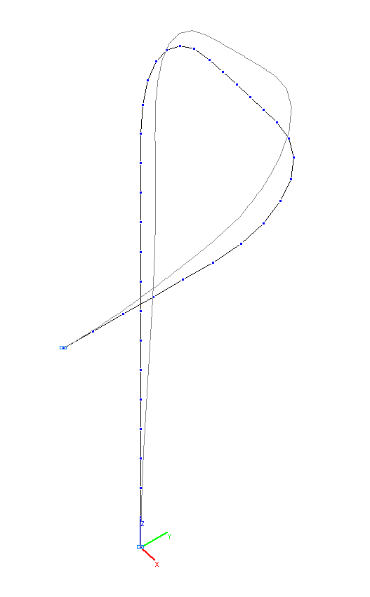
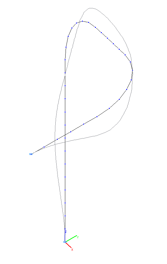
Design model
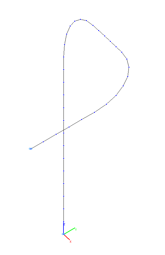
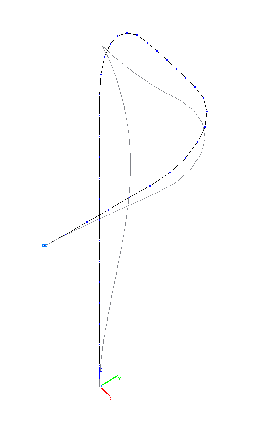
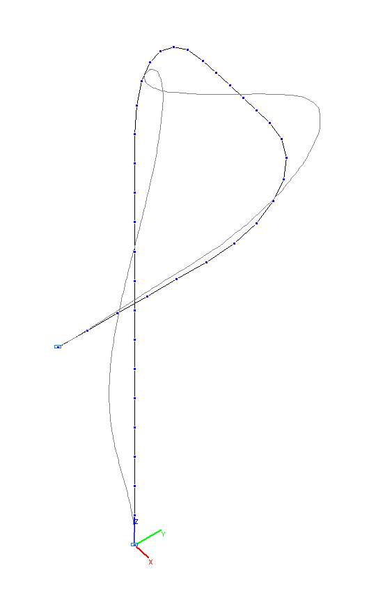
1-st and 2-nd natural oscillation modes
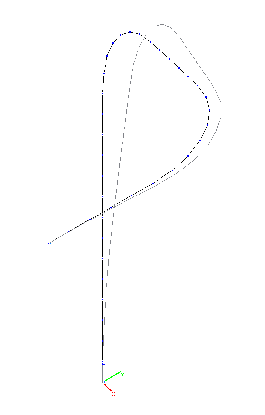
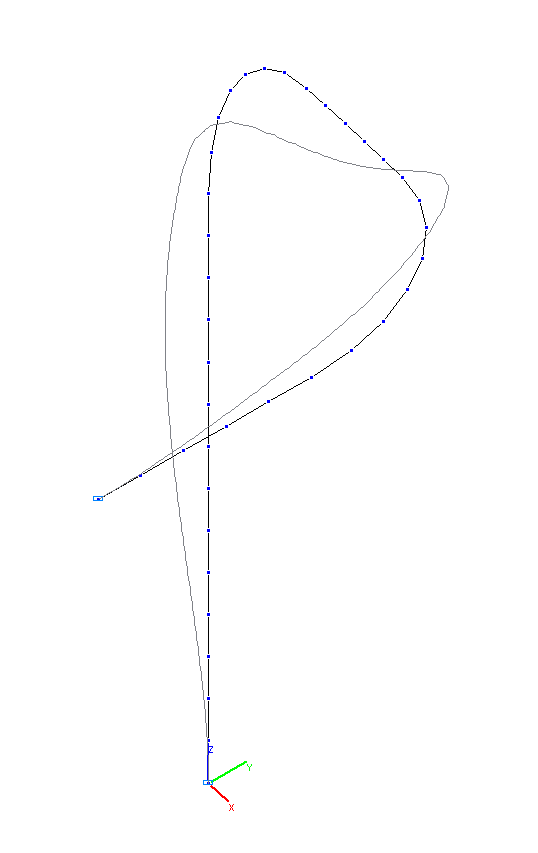
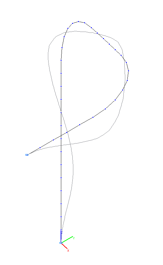
3-rd and 4-th natural oscillation modes
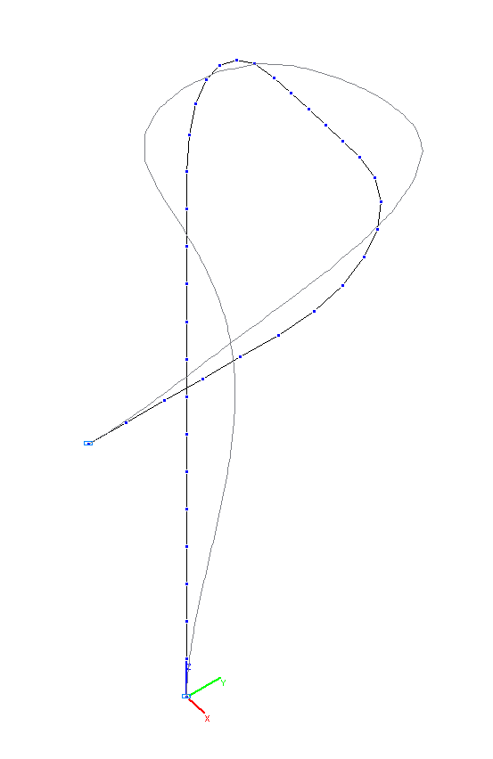
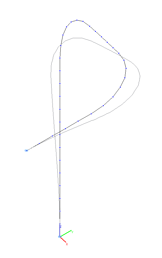
5-th and 6-th natural oscillation modes
7-th and 8-th natural oscillation modes
9-th natural oscillation mode
Comparison of solutions:
Natural frequencies f, Hz
|
Oscillation mode |
Theory |
SCAD |
Deviations, % |
|---|---|---|---|
|
1 |
10.18 |
10.01 |
1.67 |
|
2 |
19.54 |
19.29 |
1.28 |
|
3 |
25.47 |
24.55 |
3.61 |
|
4 |
48.09 |
46.79 |
2.70 |
|
5 |
52.86 |
50.77 |
3.95 |
|
6 |
75.94 |
82.21 |
8.26 |
|
7 |
80.11 |
84.29 |
5.22 |
|
8 |
122.34 |
126.58 |
3.47 |
|
9 |
123.15 |
128.51 |
4.35 |