Simply Supported Weightless Beam with Two Concentrated Masses and Transverse Sudden Constant Load Applied to One of Them

Objective: Determination of the stress-strain state of a simply supported weightless beam with two concentrated masses and transverse sudden constant load applied to one of them.
Initial data files:
5.12_Sudd_L.spr
Diagram_5.12_Sudd_L.txt
Problem formulation: Two identical loads of mass m are attached to the simply supported beam of constant cross-section at a quarter span distance from each support. The mass of the beam is neglected in comparison with the masses of the loads. The force P is applied to one of the masses at the initial time and remains constant. Determine the natural oscillation modes and natural frequencies p of the simply supported beam, as well as the deflections η and bending moments M in the cross-sections of the beam with the attached masses with time.
References: S.D. Ponomarev, V.L. Biederman, K.K. Likharev, V.M. Makushin, N.N. Malinin, V.I. Feodos’yev, Fundamentals of Modern Methods for Strength Analysis in Mechanical Engineering. Dynamic Analysis. Stability. Creep. Moscow, Mashgiz, 1952, p.150.
Initial data:
| E = 3.0·106 tf/m2 | - elastic modulus; |
| ν = 0.2 | - Poisson’s ratio; |
| b = 0.4 m | - width of the rectangular cross-section of the beam; |
| h = 0.8 m | - height of the rectangular cross-section of the beam; |
| l = 8.0 m | - beam span length; |
| m = 3.0 tf·s2/м | - value of the concentrated masses attached to the beam; |
| P = 76.8 tf | - value of the transverse sudden constant force applied to one of the masses; |
| g = 10.00 m/d2 | - gravitational acceleration; |
| I = b·h3/12 = 0.017067 | - cross-sectional moment of inertia of the beam. |
Finite element model: Design model – plane frame, 32 bar elements of type 2. Boundary conditions of the simply supported ends of the beam are provided by imposing constraints in the direction of the degree of freedom Z. The dimensional stability of the design model is provided by imposing a constraint in the node on the symmetry axis of the beam in the direction of the degree of freedom X. The concentrated masses are specified by transforming the static nodal loads m·g.
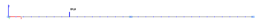
The calculation is performed in two stages: first the natural oscillation modes and natural frequencies p are determined by the modal analysis, and then the deflections η and bending moments M in the cross-sections of the beam with the attached masses with time are determined by the direct integration of the equations of motion method. The action of the transverse sudden constant force is described by the graph of the load variation with time and is given in the form of a nodal force acting along the Z axis of the global coordinate system with the scale factor of 1.0 and the delay time 0.0 s. Intervals between the time points of the load variation graph are equal to Δtint = 0.001571 c (T1/100) and correspond to the integration step. When plotting the graph, the action of the transverse sudden constant force is taken as P = 76.8 tf at all time points n·Δtint. The duration of the process is equal to t = 0.3142 s, which corresponds to twice the value of the fundamental period of oscillations 2·T1. Critical damping ratios for the 1-st and 2-nd natural frequencies are taken with the minimum value ξ = 0.0001. The conversion factor for the added static loading is equal to k = 0.981 (mass generation). Number of nodes in the design model – 33. The modal integration method is used in the calculation. The determination of the natural oscillation modes and natural frequencies is performed by the method of subspace iteration. The matrix of concentrated masses is used in the calculation.
Results in SCAD
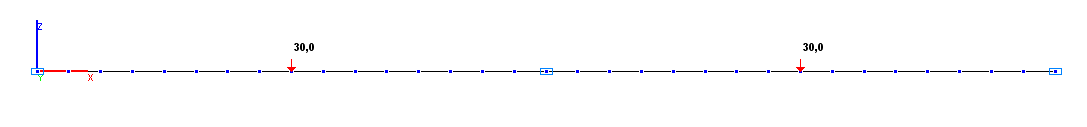
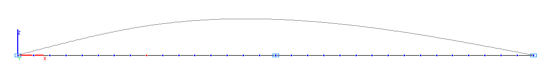
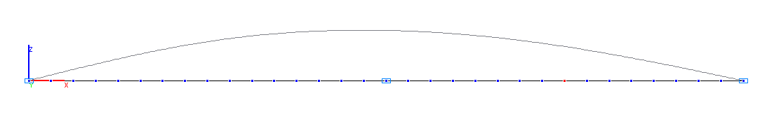
Design model
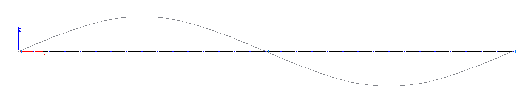
1-st and 2-nd natural oscillation modes
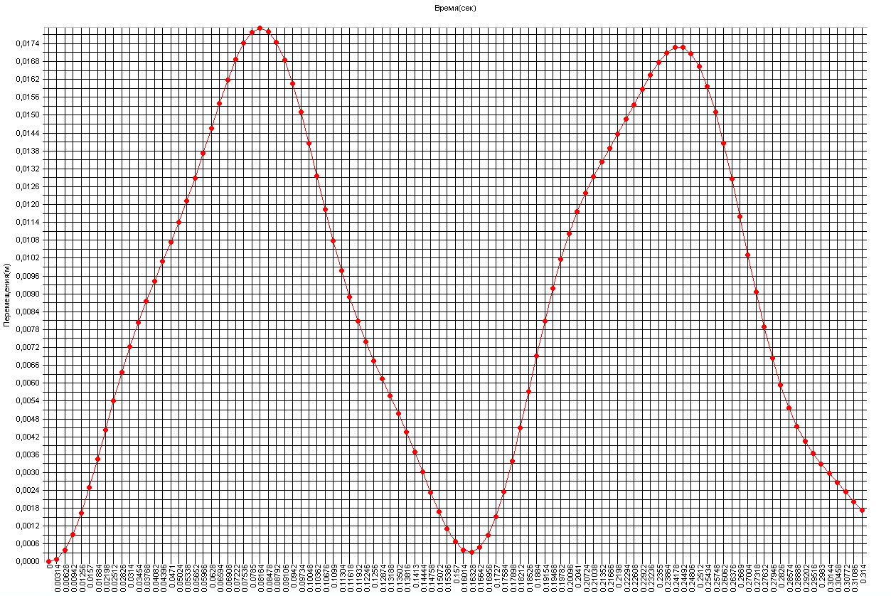
Graph of the variation of the deflection η1 in the cross-section of the beam
with the attached mass subjected to the shear force with time (m)
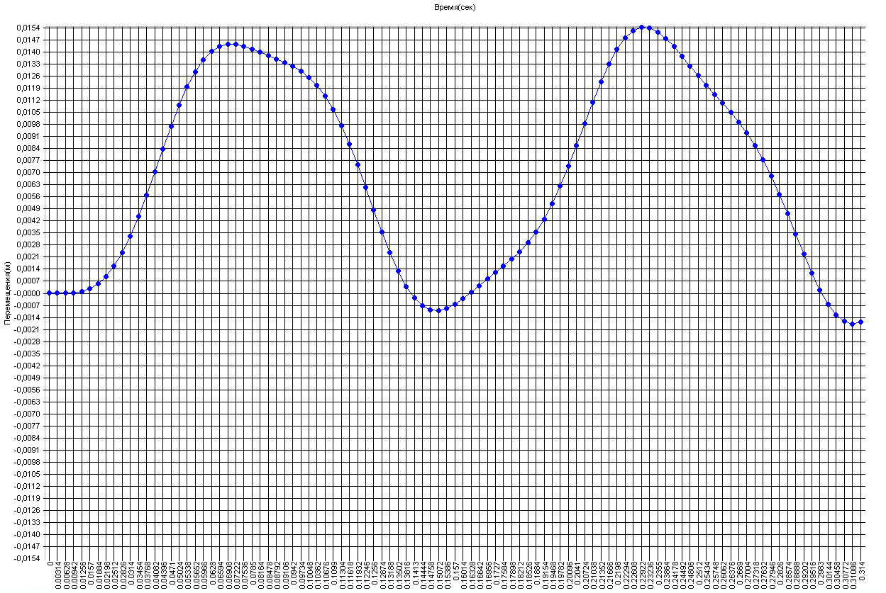
Graph of the variation of the deflection η2 in the cross-section of the beam
with the attached mass not subjected to the shear force with time (m)
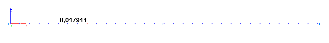
Amplitude value of the deflection η1 in the cross-section of the beam
with the attached mass subjected to the shear force and the deformed model at the respective time point (m)
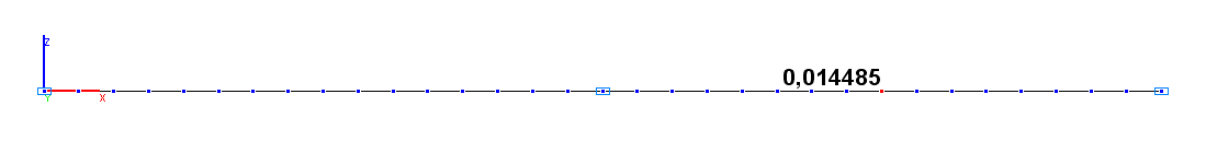
Amplitude value of the deflection η2 in the cross-section of the beam
with the attached mass not subjected to the shear force and the deformed model at the respective time point (m)
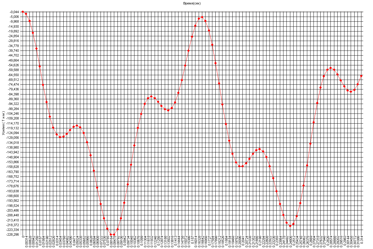
Graph of the variation of the bending moment M1 in the cross-section of the beam
with the attached mass subjected to the shear force, with time (tm·m)
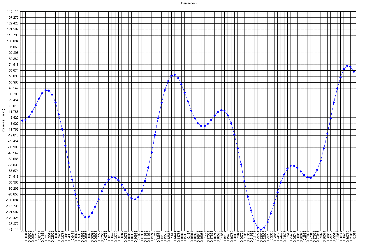
Graph of the variation of the bending moment M2 in the cross-section of the beam
with the attached mass not subjected to the shear force, with time (tm·m)
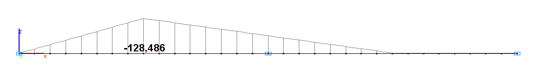
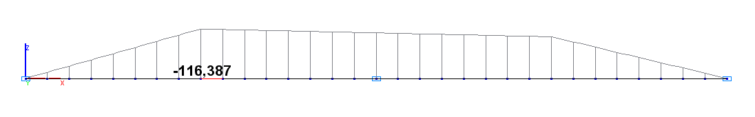
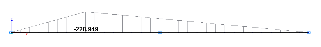
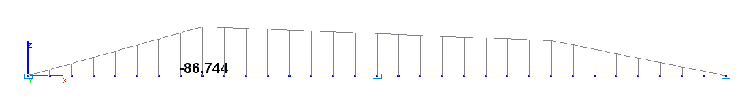
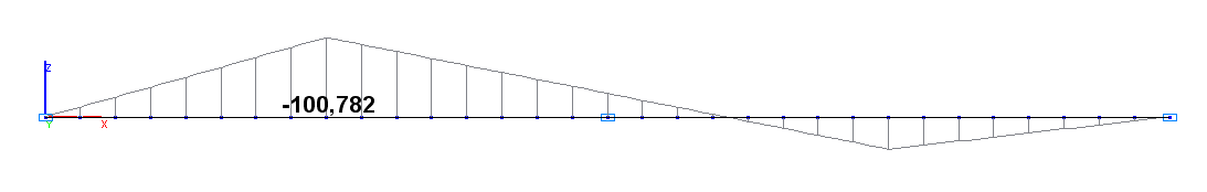
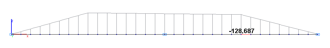
Amplitude values of the bending moment M1 in the cross-section of the beam
with the attached mass subjected to the shear force (tm·m)
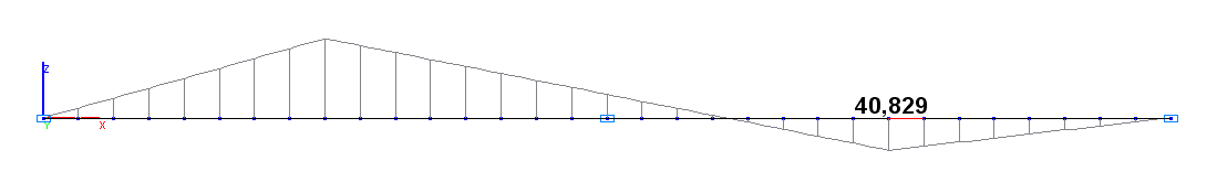
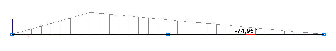
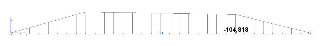
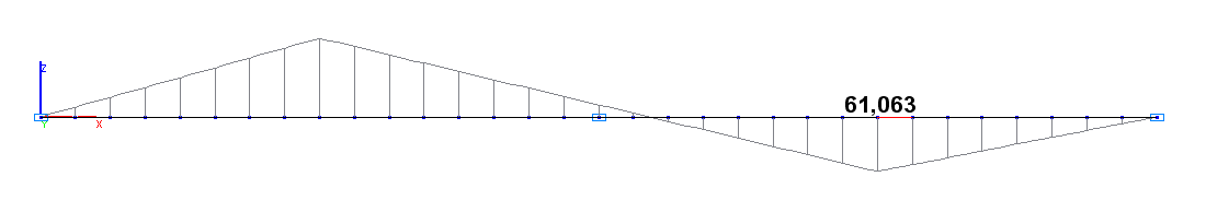
Amplitude values of the bending moment M2 in the cross-section of the beam
with the attached mass not subjected to the shear force (tm·m)
Comparison of solutions:
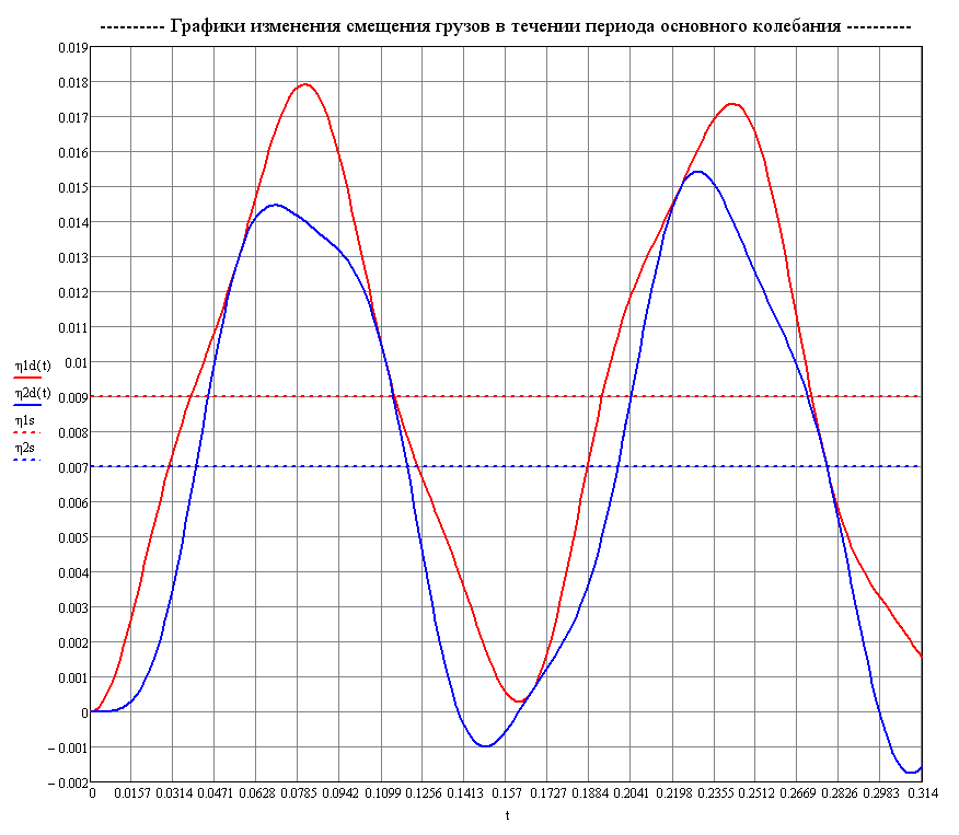
The dashed lines show the values of static deflections
Graphs of the variation of the deflections η1 and η2 in the cross-sections of the beam
with the attached masses with time according to the theoretical solution (m)
The dashed lines show the values of static bending moments
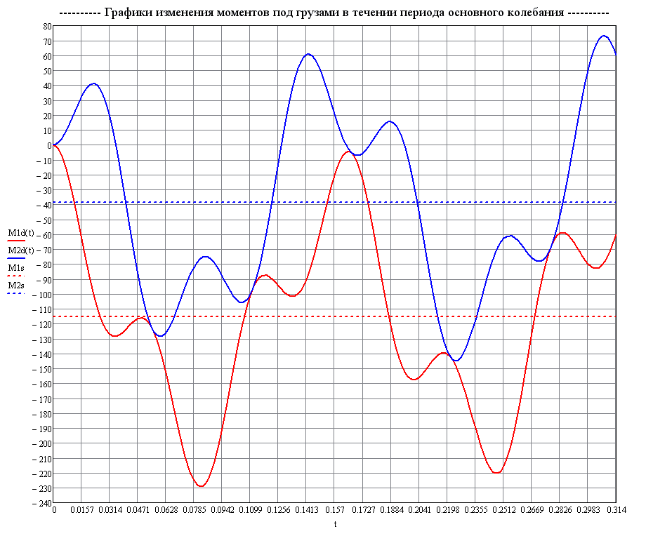
Graphs of the variation of the bending moments M1 and M2 in the cross-sections of the beam
with the attached masses with time according to the theoretical solution (tf·m)
Natural frequencies p, rad/s
|
Oscillation mode |
Theory |
SCAD |
Deviations, % |
|---|---|---|---|
|
1 |
40.000 |
40.000 |
0.00 |
|
2 |
113.137 |
113.137 |
0.00 |
Amplitude value of the deflections η in the cross-sections of the beam
with the attached masses, m
|
Nodal mass |
Theory |
SCAD |
|||
|---|---|---|---|---|---|
|
Time, s |
Deflection, m |
Time, s |
Deflection, m |
Deviations, % |
|
|
1 |
0.0809 |
0.017928 |
0.0817 |
0.017911 |
0.09 |
|
2 |
0.0695 |
0.014474 |
0.0707 |
0.014485 |
0.08 |
Amplitude value of the bending moments M in the cross-sections of the beam
with the attached masses, tf·m
|
Nodal mass |
Theory |
SCAD |
|||
|---|---|---|---|---|---|
|
Time, s |
Bending moment, tf·m |
Time, s |
Bending moment, tf·m |
Deviations, % |
|
|
1 |
0.0346 |
-128.426 |
0.0361 |
-128.486 |
0.05 |
|
1 |
0.0493 |
-115.960 |
0.0503 |
-116.387 |
0.37 |
|
1 |
0.0824 |
-229.286 |
0.0833 |
-228.949 |
0.15 |
|
1 |
0.1180 |
-87.419 |
0.1194 |
-86.744 |
0.77 |
|
1 |
0.1334 |
-101.705 |
0.1351 |
-100.782 |
0.91 |
|
2 |
0.0226 |
+41.120 |
0.0236 |
+40.829 |
0.71 |
|
2 |
0.0599 |
-128.638 |
0.0613 |
-128.687 |
0.04 |
|
2 |
0.0849 |
-74.952 |
0.0864 |
-74.957 |
0.01 |
|
2 |
0.1052 |
-105.748 |
0.1068 |
-104.818 |
0.88 |
|
2 |
0.1423 |
+60.864 |
0.1430 |
+61.063 |
0.33 |
Notes: In the analytical solution the natural frequencies of oscillations p of the simply supported beam are determined according to the following formulas:
\[ p_{1} =\sqrt {\frac{48\cdot E\cdot I}{m\cdot l^{3}}} ; \quad p_{2} =\sqrt {\frac{384\cdot E\cdot I}{m\cdot l^{3}}} . \]
In the analytical solution the deflections η in the cross-sections of the beam with the attached masses with time are determined according to the following formulas:
\[ \eta_{1} \left( t \right)=\frac{P\cdot l^{3}}{768\cdot E\cdot I}\cdot \left[ {8\cdot \left( {1-\cos \left( {p_{1} \cdot t} \right)} \right)+\left( {1-\cos \left( {p_{2} \cdot t} \right)} \right)} \right]; \] \[ \eta_{2} \left( t \right)=\frac{P\cdot l^{3}}{768\cdot E\cdot I}\cdot \left[ {8\cdot \left( {1-\cos \left( {p_{1} \cdot t} \right)} \right)-\left( {1-\cos \left( {p_{2} \cdot t} \right)} \right)} \right]. \]
In the analytical solution the bending moments M in the cross-sections of the beam with the attached masses with time are determined according to the following formulas:
\[ \eta_{1} \left( t \right)=\frac{P\cdot l^{3}}{768\cdot E\cdot I}\cdot \left[ {8\cdot \left( {1-\cos \left( {p_{1} \cdot t} \right)} \right)+\left( {1-\cos \left( {p_{2} \cdot t} \right)} \right)} \right]; \] \[ \eta_{2} \left( t \right)=\frac{P\cdot l^{3}}{768\cdot E\cdot I}\cdot \left[ {8\cdot \left( {1-\cos \left( {p_{1} \cdot t} \right)} \right)-\left( {1-\cos \left( {p_{2} \cdot t} \right)} \right)} \right]. \]