Simply Supported Beam with a Distributed Mass Subjected to a Transverse Harmonic Exciting Force Applied in the Middle of the Span

Objective: Determination of the strain state of a simply supported beam with a distributed mass subjected to a transverse harmonic exciting force applied in the middle of the span.
Initial data file:
5.13.spr,
Diagram_5.13.txt
Problem formulation: The force P0 is applied in the middle of the span of the simply supported beam of constant cross-section with the uniformly distributed mass μ at the initial time and varies harmonically with the frequency ω. Determine the natural oscillation modes and natural frequencies p of the simply supported beam, as well as the deflection η in the cross-section in the middle of the beam span with time.
References: Timoshenko S.P., Course of the Theory of Elasticity, Kiev, Naukova Dumka, 1972, p. 343.
Initial data:
| E = 3.0·106 tf/m2 | - elastic modulus; |
| ν = 0.2 | - Poisson’s ratio; |
| b = 0.4 m | - width of the rectangular cross-section of the beam; |
| h = 0.8 m | - height of the rectangular cross-section of the beam; |
| l = 8.0 m | - beam span length; |
| γ = 2.5 tf/m3 | - specific weight of the beam material; |
| P0 = 76.8 tf | - amplitude value of the harmonic exciting force applied in the middle of the span; |
| g = 10.00 m/s2 | - gravitational acceleration; |
| μ = 2.5·0.4·0.8/10.0 = 0.08 tf·s2/m2 | - value of the uniformly distributed mass of the beam; |
| I = 0.4·(0.8)3/12 = 0.017067 m4 | - cross-sectional moment of inertia of the beam. |
The frequency of the harmonic exciting force ω is taken depending on the value of the fundamental natural frequency of the beam p1:
ω = 0.5·p1.
Finite element model: Design model – grade beam / plate, 32 bar elements of type 3. Boundary conditions of the simply supported ends of the beam are provided by imposing constraints in the direction of the degree of freedom Z. The dimensional stability of the design model is provided by imposing a constraint in the node of the cross-section along the symmetry axis of the beam in the direction of the degree of freedom UX. The distributed mass is specified by transforming the static load from the self-weight of the beam μ·g.
The calculation is performed in two stages: first the natural oscillation modes and natural frequencies p are determined by the modal analysis, and then the deflections η in the cross-section in the middle of the beam span with time are determined by the direct integration of the equations of motion method. The action of the transverse harmonic exciting force is described by the graph of the load variation with time and is given in the form of a nodal force acting along the Z axis of the global coordinate system with the scale factor of 1.0 and the delay time 0.0 s. Intervals between the time points of the load variation graph are equal to Δtint = T/100, where T – period of the harmonic exciting force, and correspond to the integration step. When plotting the graph, the action of the transverse harmonic exciting force is taken as Pn = P0·cos(ω·n·Δtint) at the time points n·Δtint. The duration of the process is equal to t = 2·T. Critical damping ratios for the 1-st and 2-nd natural frequencies are taken with the minimum value ξ = 0.0001. The conversion factor for the added static loading is equal to k = 0.981 (mass generation). Number of nodes in the design model – 33. The modal integration method is used in the calculation. The determination of the natural oscillation modes and natural frequencies is performed by the method of subspace iteration. The matrix of concentrated masses is used in the calculation.
Results in SCAD


Design model
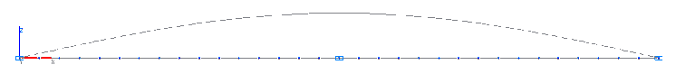
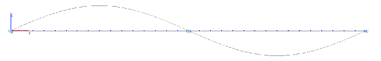
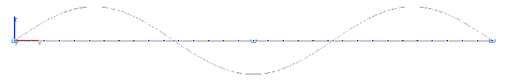
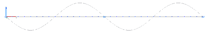
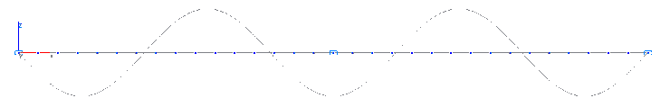
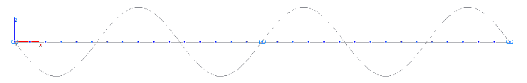
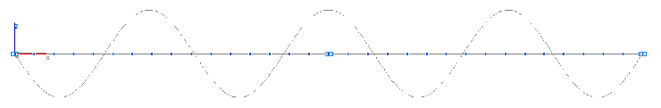
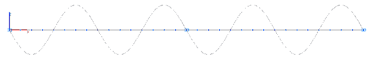
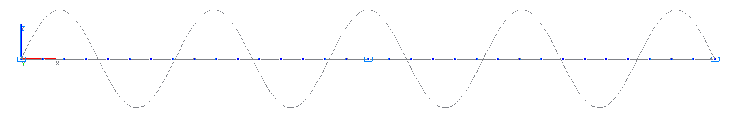
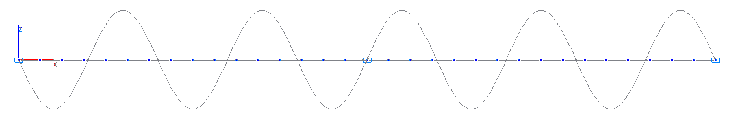
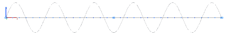
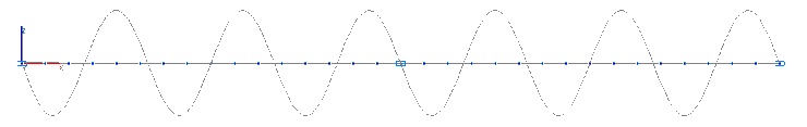
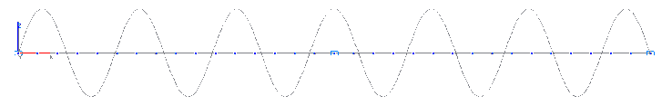
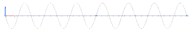
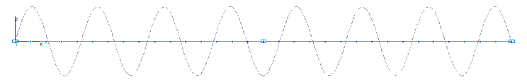
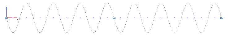
1-st -- 16-th natural oscillation modes
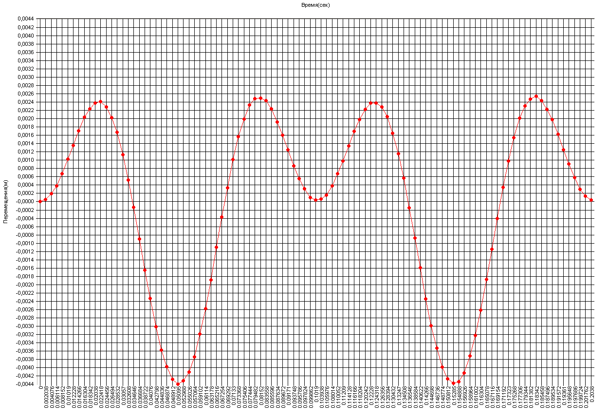
Graph of the variation of the deflection η in the cross-section in the middle of the beam span with time (m).


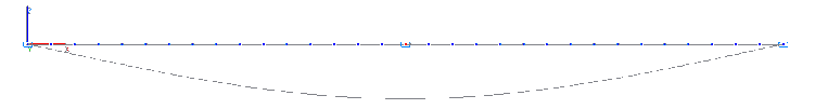


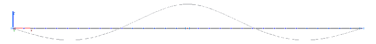


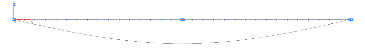


Amplitude values of the deflection η in the cross-section in the middle of the beam span and the deformed models at the respective time points (m).
Comparison of solutions:
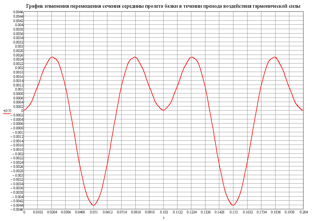
Graph of the variation of the deflection η in the cross-section in the middle of the beam span with time according to the theoretical solution (m)
Natural frequencies p, rad/s
|
Oscillation mode |
Theory |
SCAD |
Deviations, % |
|---|---|---|---|
|
1 |
123.370 |
123.370 |
0.00 |
|
2 |
493.480 |
493.480 |
0.00 |
|
3 |
1110.330 |
1110.325 |
0.00 |
|
4 |
1973.921 |
1973.887 |
0.00 |
|
5 |
3084.251 |
3084.120 |
0.00 |
|
6 |
4441.322 |
4440.919 |
0.01 |
|
7 |
6045.133 |
6044.087 |
0.02 |
|
8 |
7895.684 |
7893.275 |
0.03 |
|
9 |
9992.974 |
9987.907 |
0.05 |
|
10 |
12337.005 |
12327.069 |
0.08 |
|
11 |
14927.777 |
14909.367 |
0.12 |
|
12 |
17765.288 |
17732.721 |
0.18 |
|
13 |
20849.539 |
20794.097 |
0.27 |
|
14 |
24180.531 |
24089.155 |
0.38 |
|
15 |
27758.262 |
27611.778 |
0.53 |
|
16 |
31582.734 |
31353.470 |
0.73 |
Amplitude values of the deflection η in the cross-section in the middle of the beam span
at the frequency of the harmonic exciting force ω = 0.5·p1
|
Theory |
SCAD |
|||
|---|---|---|---|---|
|
Time, s |
Deflection, m |
Time, s |
Deflection, m |
Deviations, % |
|
0.0210 |
0.002474 |
0.0224 |
0.002421 |
2.14 |
|
0.0510 |
-0.004428 |
0.0510 |
-0.004410 |
0.41 |
|
0.0809 |
0.002474 |
0.0815 |
0.002504 |
1.21 |
|
0.1017 |
0.000002 |
0.1019 |
0.000040 |
─ |
|
0.1228 |
0.002474 |
0.1223 |
0.002383 |
3.68 |
|
0.1528 |
-0.004428 |
0.1529 |
-0.004374 |
1.22 |
|
0.1828 |
0.002474 |
0.1834 |
0.002547 |
2.95 |
Notes: In the analytical solution the natural frequencies of oscillations p of the simply supported beam are determined according to the following formulas:
\[ \frac{n^{2}\cdot \pi^{2}}{l^{2}}\cdot \sqrt {\frac{E\cdot I}{\mu }} , \]
where n = 1, 2, 3, 4, … – natural mode number.
In the analytical solution the deflections η in the cross-sections in the middle of the beam span with time are determined according to the following formula:
\[ \eta \left( t \right)=\frac{2\cdot P_{0} \cdot l^{3}}{\pi^{4}\cdot E\cdot I}\cdot \sum\limits_{n=1} {\left[ {\frac{\left( {\sin \left( {\frac{n\cdot \pi }{2}} \right)} \right)^{2}}{n^{4}\cdot \left( {1-\frac{\mu \cdot l^{4}\cdot \omega^{2}}{n^{4}\cdot \pi^{4}\cdot E\cdot I}} \right)}\cdot \left( {\cos \left( {\omega \cdot t} \right)-\cos \left( {\frac{n^{2}\cdot \pi^{2}}{l^{2}}\cdot \sqrt {\frac{E\cdot I}{\mu }} \cdot t} \right)} \right)} \right]} ; \]