Natural Oscillations of a Clamped Square Plate

Objective: Modal analysis of a clamped square plate.
Initial data file: 5.4.spr
Problem formulation: Determine the natural oscillation modes and frequencies ω of the clamped square plate with the density of the material ρ.
References: I.A. Birger, Ya.G. Panovko, Strength, Stability, Vibrations, Handbook in three volumes, Volume 3, Moscow, Mechanical engineering, 1968, p. 377.
Initial data:
| E = 2.06·108 kPa | - elastic modulus; |
| ν = 0.3 | - Poisson’s ratio; |
| ρ = 7.85 t/m3 | - density of the material; |
| h = 0.01 m | - thickness of the plate; |
| a1 = 1.0 m | - long side of the plate (along the X axis of the global coordinate system); |
| a2 = 1.0 m | - short side of the plate (along the Y axis of the global coordinate system). |
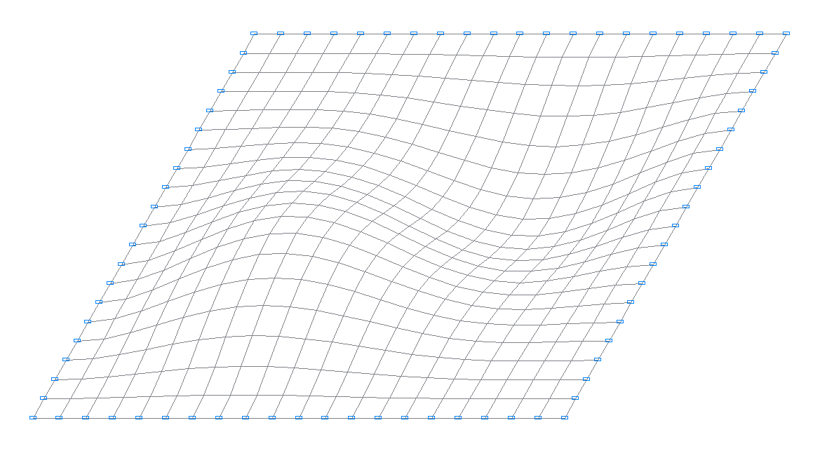
Finite element model: Design model – grade beam / plate, 400 plate elements of type 20. The spacing of the finite element mesh along the sides of the plate (along the X, Y axes of the global coordinate system) is 0.05 m. Boundary conditions are provided by imposing constraints in the directions of the degrees of freedom Z, UX, UY for the edges parallel to the X and Y axes of the global coordinate system. The distributed mass is specified by transforming the static load from the self-weight of the plate ow = γ∙h, where γ = ρ∙g = 77.01 kN/m3. Number of nodes in the design model – 441. The determination of the natural oscillation modes and natural frequencies is performed by the method of subspace iteration. The matrix of concentrated masses is used in the calculation.
Results in SCAD
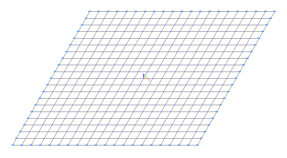
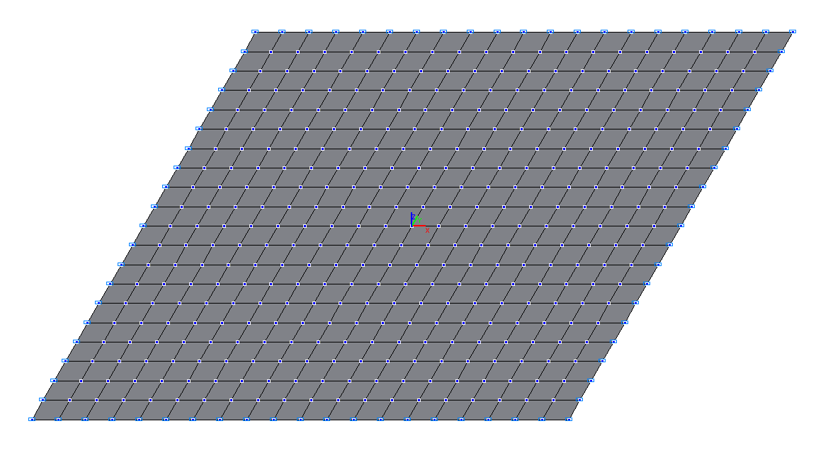
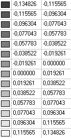
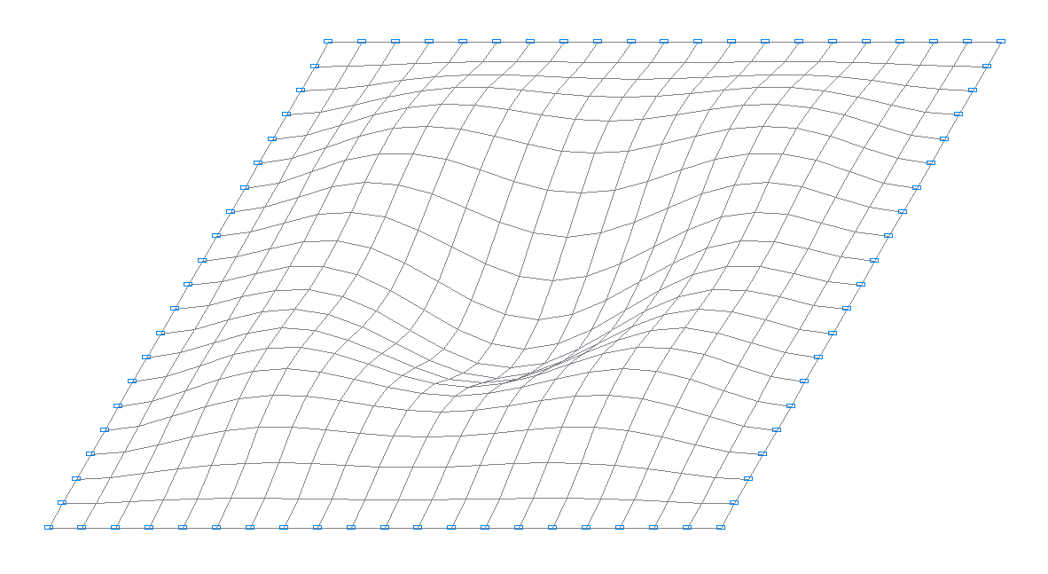
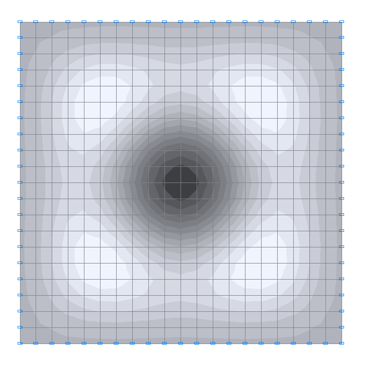
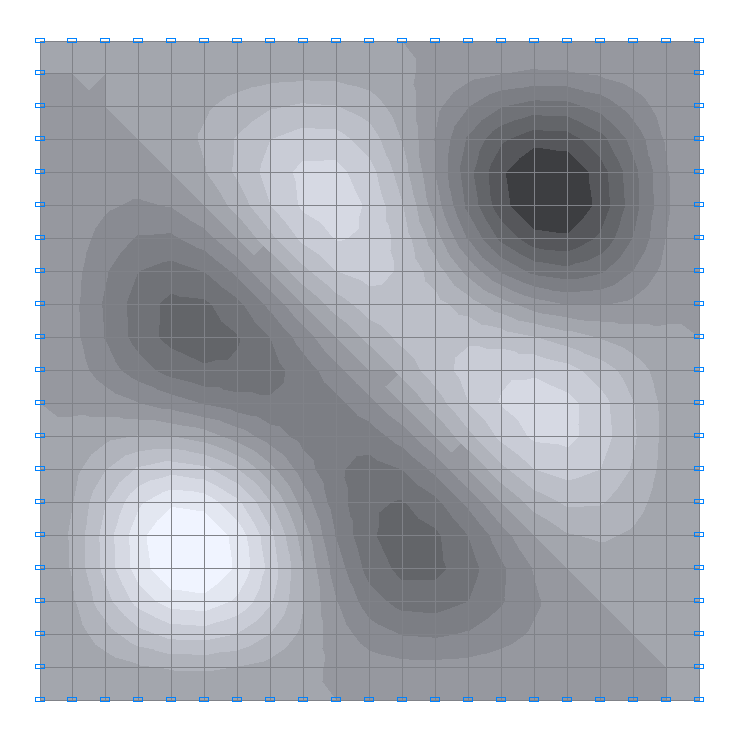
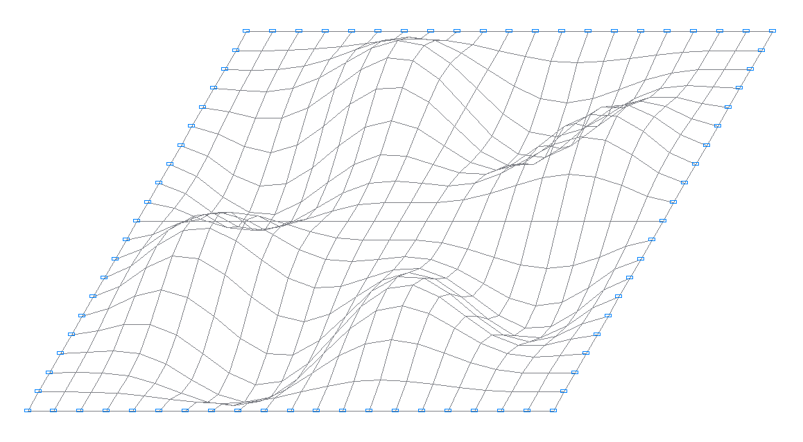
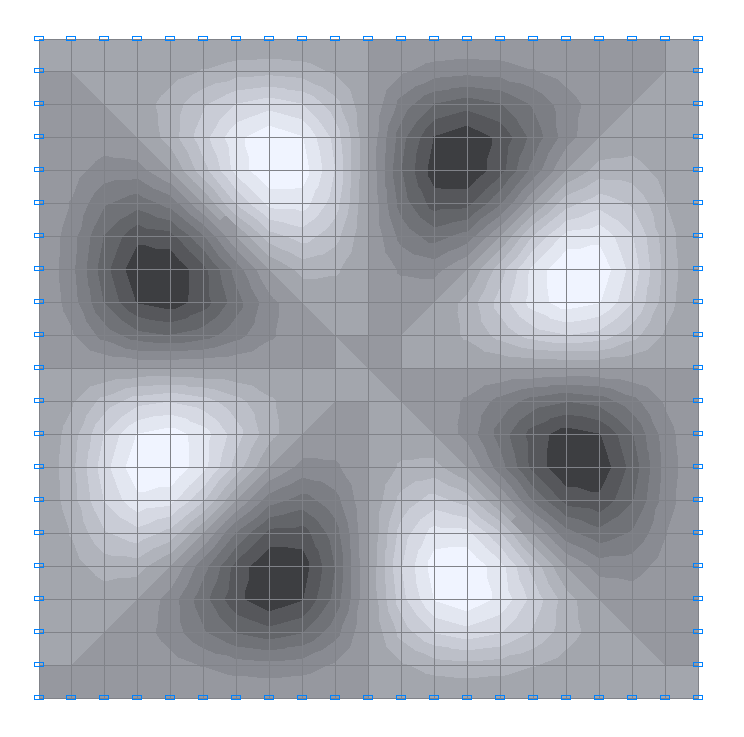
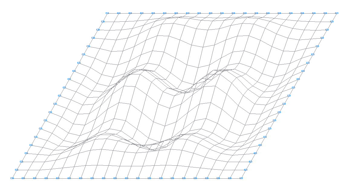
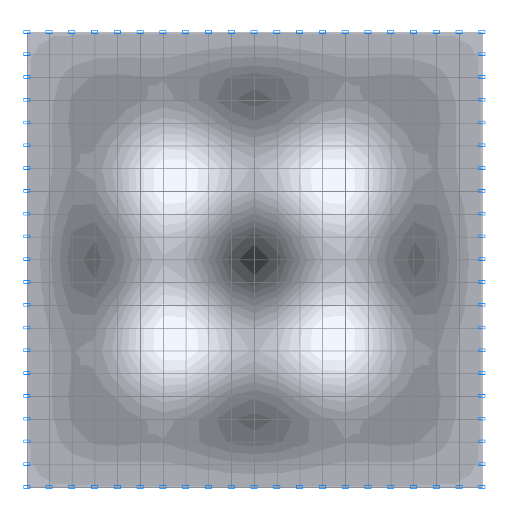
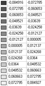
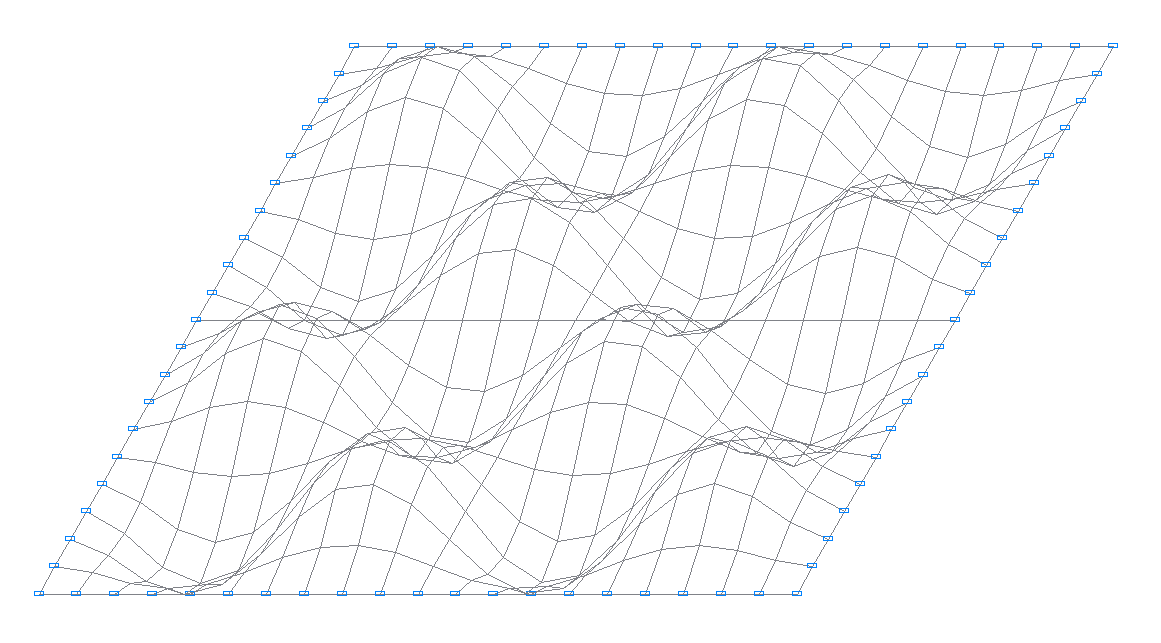
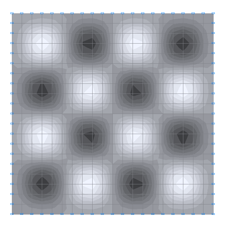
Design model
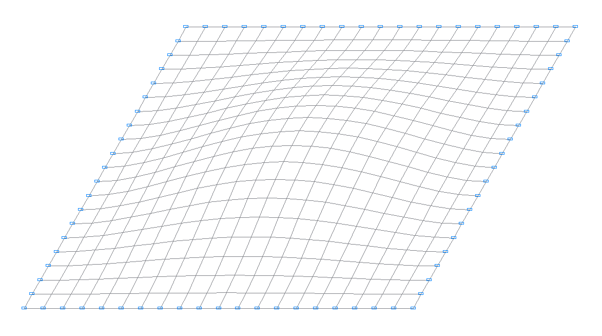
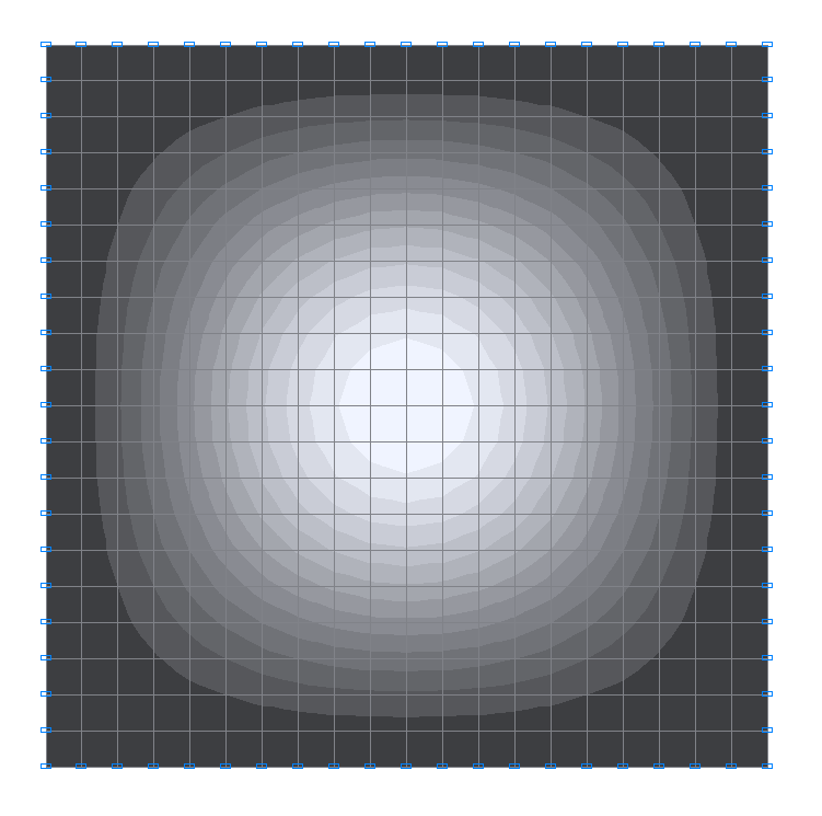
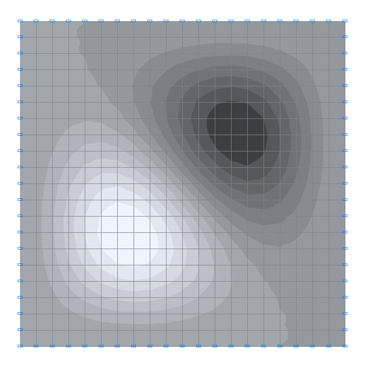
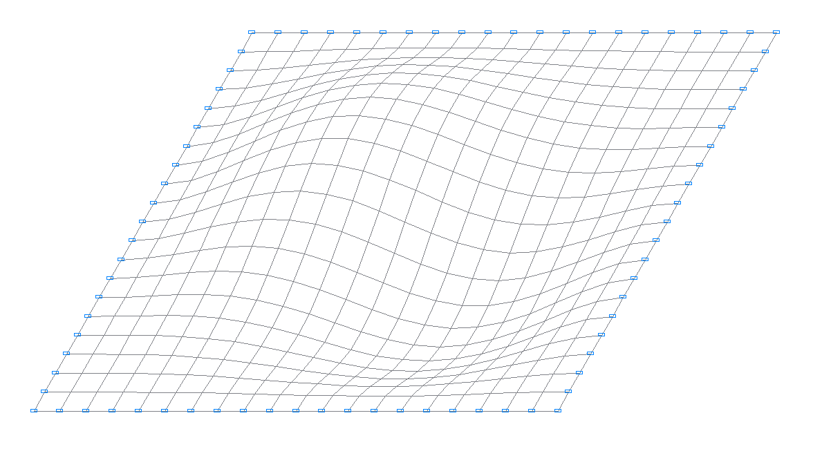
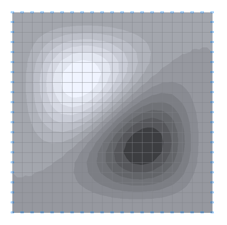
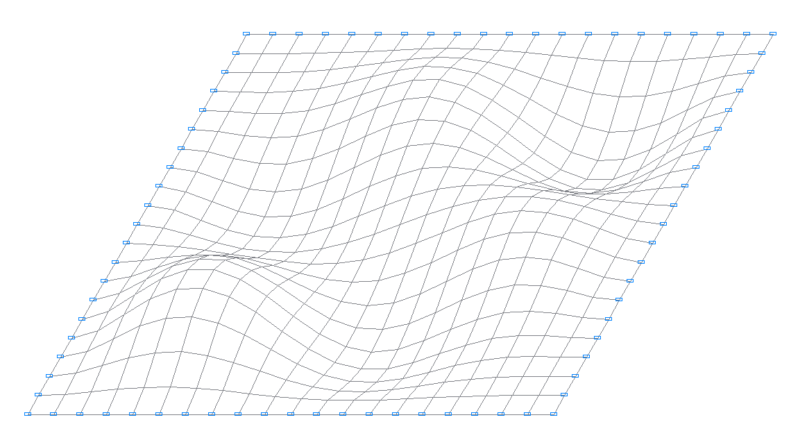
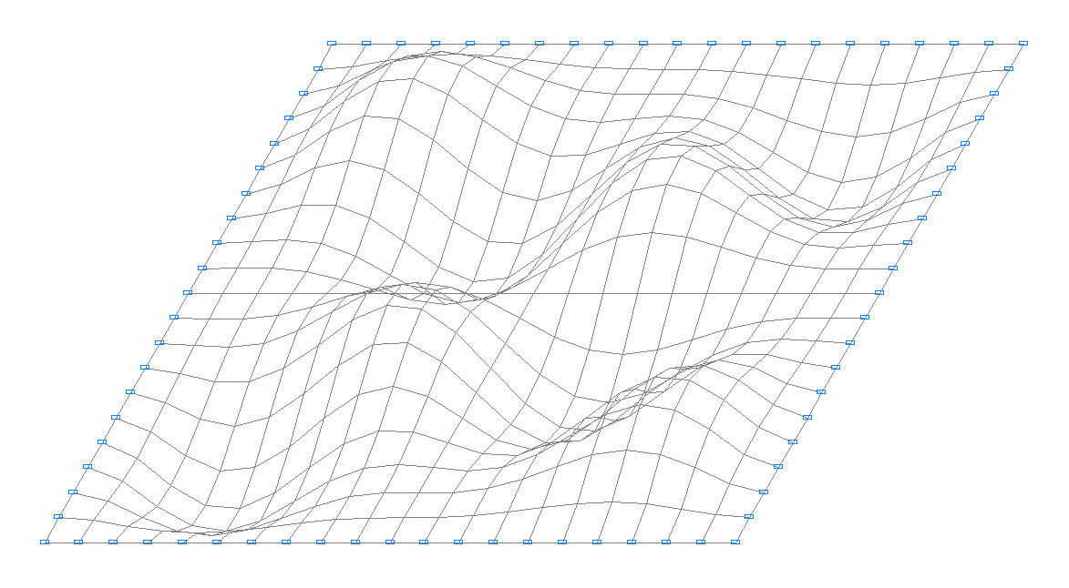
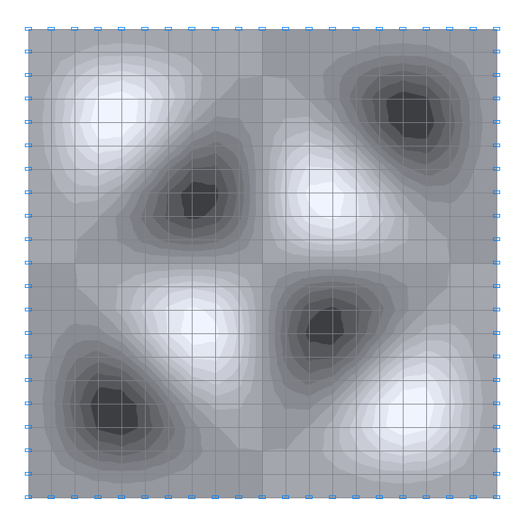
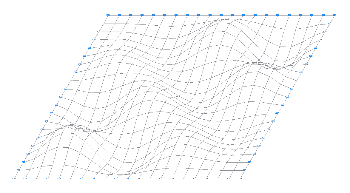
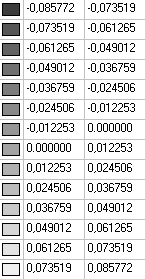
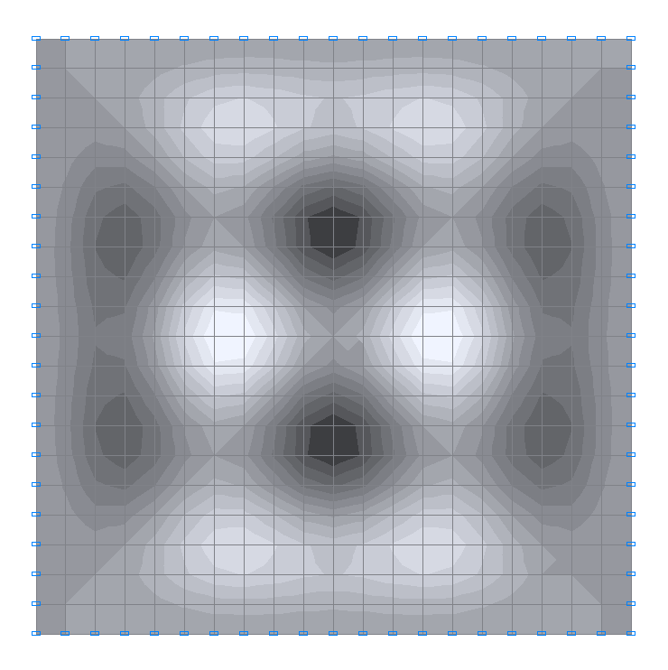
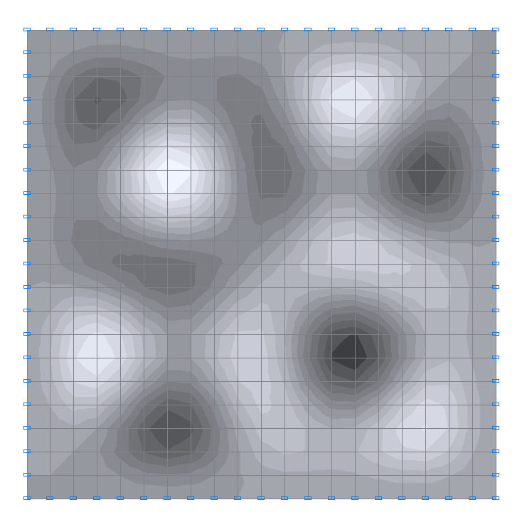
1-st natural oscillation mode
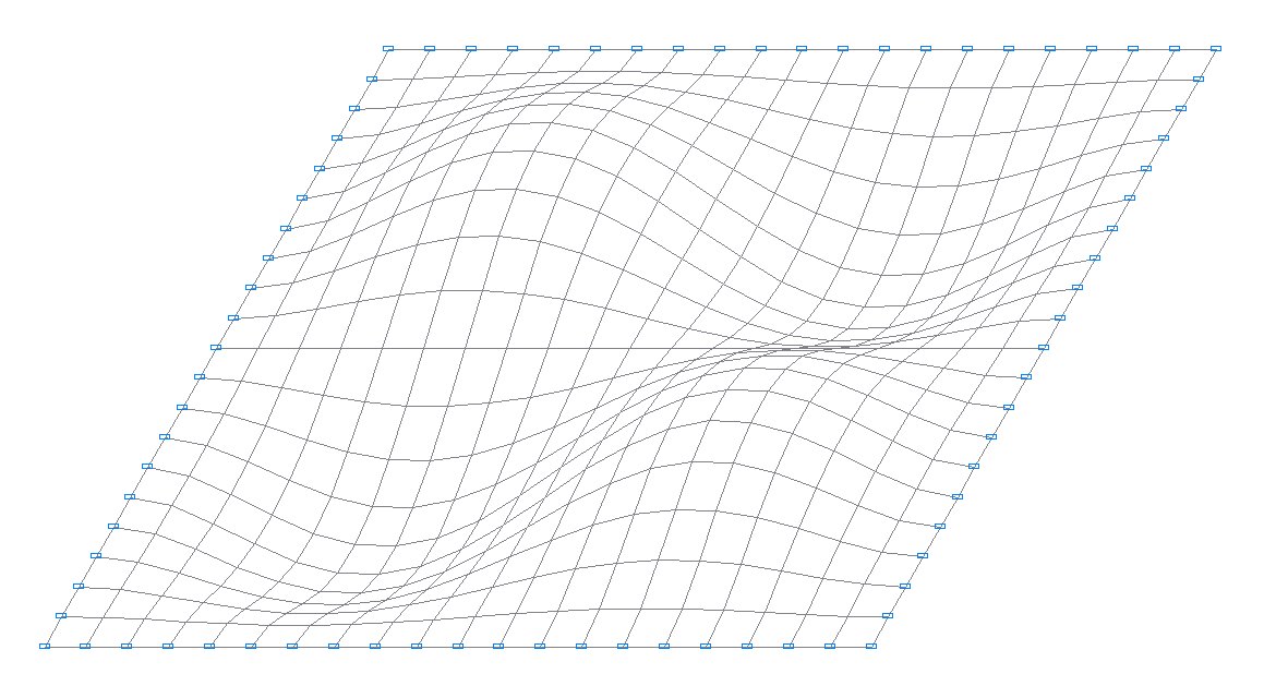
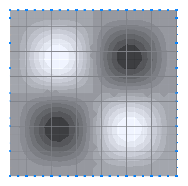
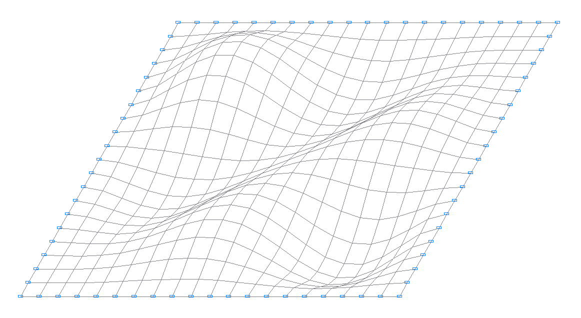
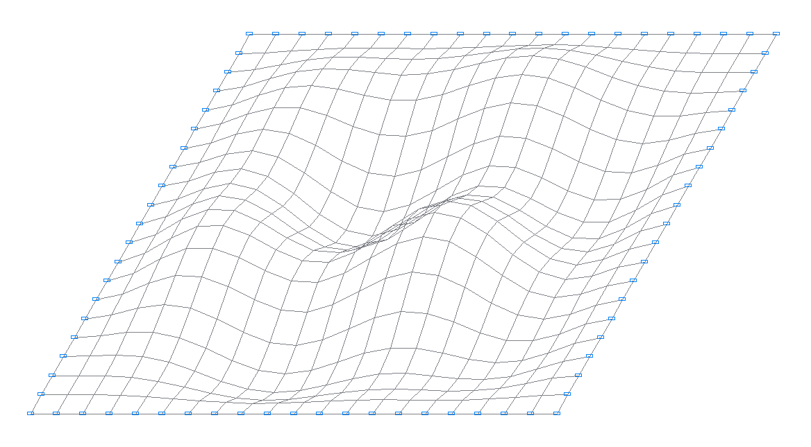
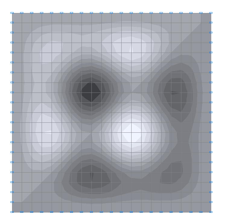
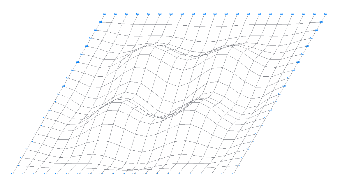
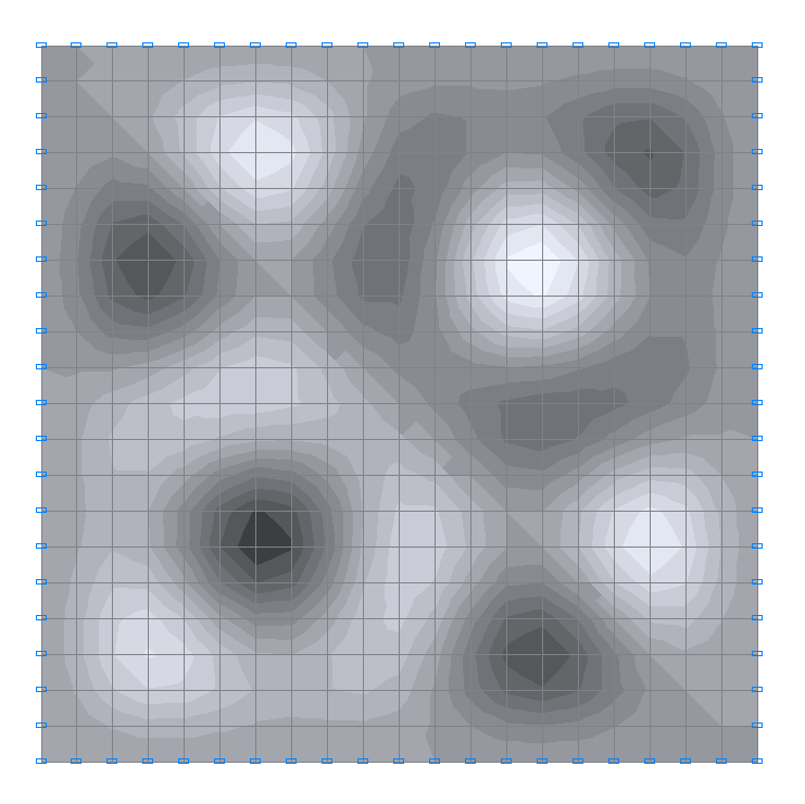
2-nd natural oscillation mode
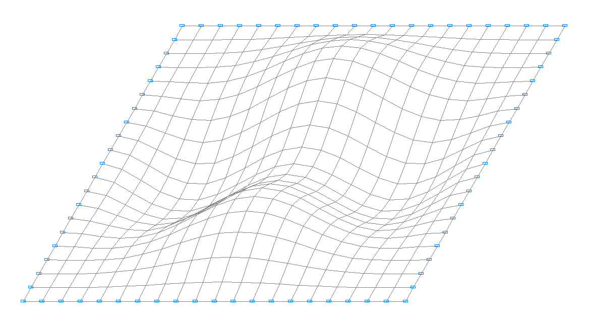
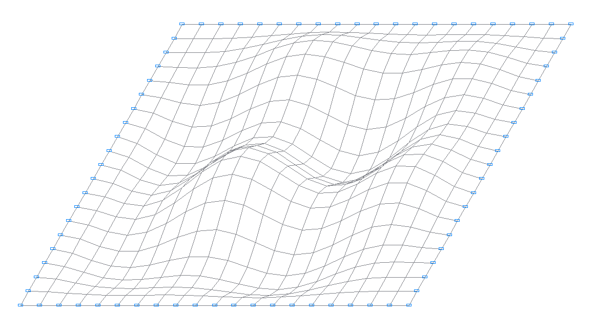
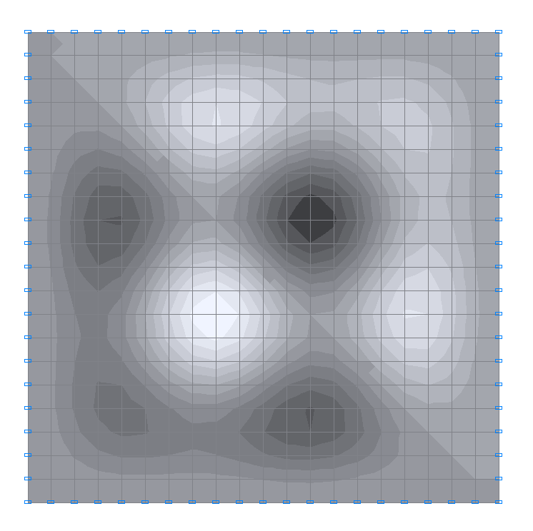
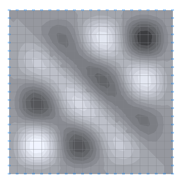
3-rd natural oscillation mode
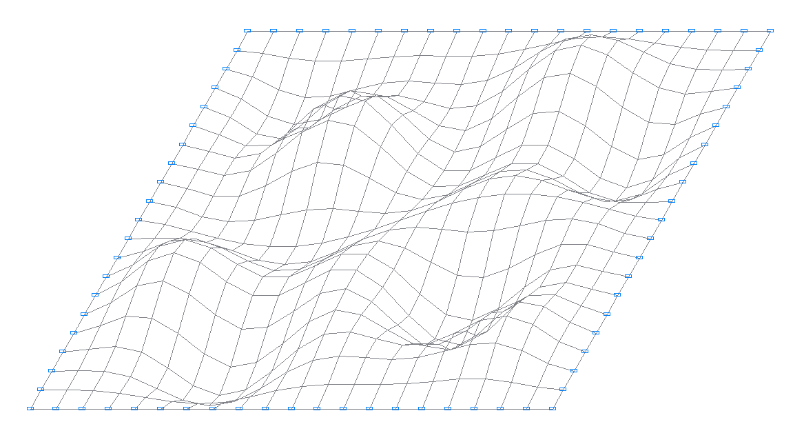
4-th natural oscillation mode
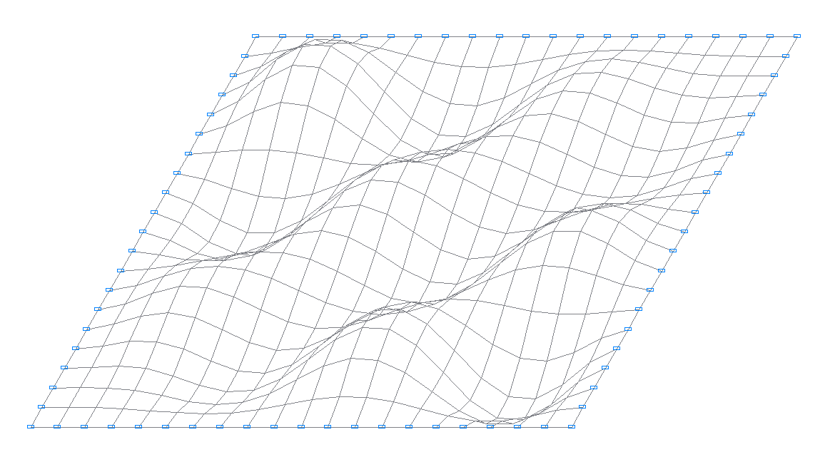
5-th natural oscillation mode
6-th natural oscillation mode

7-th natural oscillation mode

8-th natural oscillation mode
9-th natural oscillation mode
10-th natural oscillation mode
11-th natural oscillation mode
12-th natural oscillation mode
13-th natural oscillation mode
14-th natural oscillation mode
15-th natural oscillation mode
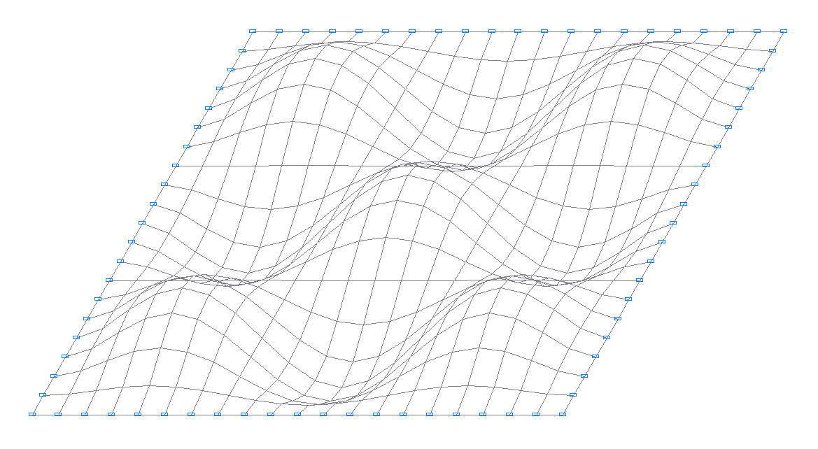
16-th natural oscillation mode
17-th natural oscillation mode
18-th natural oscillation mode
19-th natural oscillation mode
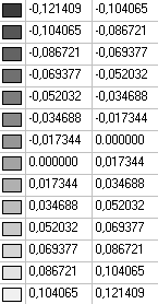
20-th natural oscillation mode
Comparison of solutions:
Natural frequencies ω, rad / s
|
Oscillation mode |
Number of half waves m1, m2 |
Theory |
SCAD |
Deviations, % |
|---|---|---|---|---|
|
1 |
1, 1 |
560.1 |
558.5 |
0.29 |
|
2 |
1, 2 |
1143.2 |
1139.4 |
0.33 |
|
3 |
2, 1 |
1143.2 |
1139.4 |
0.33 |
|
4 |
2, 2 |
1686.6 |
1683.4 |
0.19 |
|
5 |
1, 3 |
2054.0 |
2042.8 |
0.55 |
|
6 |
3, 1 |
2054.0 |
2052.2 |
0.09 |
|
7 |
2, 3 |
2571.5 |
2569.1 |
0.09 |
|
8 |
3, 2 |
2571.5 |
2569.1 |
0.09 |
|
9 |
1, 4 |
3276.5 |
3267.5 |
0.27 |
|
10 |
4, 1 |
3276.5 |
3267.5 |
0.27 |
|
11 |
3, 3 |
3424.6 |
3434.5 |
0.29 |
|
12 |
2, 4 |
3782.2 |
3772.0 |
0.27 |
|
13 |
4, 2 |
3782.2 |
3786.2 |
0.11 |
|
14 |
3, 4 |
4611.8 |
4632.3 |
0.44 |
|
15 |
4, 3 |
4611.8 |
4632.3 |
0.44 |
|
16 |
1, 5 |
4806.6 |
4793.0 |
0.28 |
|
17 |
5, 1 |
4806.6 |
4796.7 |
0.21 |
|
18 |
2, 5 |
5307.4 |
5303.5 |
0.07 |
|
19 |
5, 2 |
5307.4 |
5303.5 |
0.07 |
|
20 |
4, 4 |
5774.8 |
5821.8 |
0.81 |
Notes: In the analytical solution the natural frequencies ω of the clamped square plate with the density of the material ρ can be determined according to the following formula obtained on the basis of the Rayleigh-Ritz method:
\[\omega =\pi^{2}\cdot \left( {\frac{D}{\rho \cdot h}\cdot \left( {\frac{A_{m}^{4}}{a_{1}^{4}}+\frac{A_{n}^{4}}{a_{2}^{4}}+2\cdot \frac{B_{m} \cdot B_{n} }{a_{1}^{2}\cdot a_{2}^{2}}} \right)} \right)^{\frac{1}{2}}, \quad where: \] \[ A_{m} =\left\{ {{\begin{array}{*{20}c} {1.506} & {m=1} \\ {m+0.5} & {m\ge 2} \\ \end{array} }} \right., \quad A_{n} =\left\{ {{\begin{array}{*{20}c} {1.506} & {n=1} \\ {n+0.5} & {n\ge 2} \\ \end{array} }} \right., \quad B_{m} =\left\{ {{\begin{array}{*{20}c} {1.248} & {m=1} \\ {A_{m} \cdot \left( {A_{m} -\frac{2}{\pi }} \right)} & {m\ge 2} \\ \end{array} }} \right., \quad B_{m} =\left\{ {{\begin{array}{*{20}c} {1.248} & {n=1} \\ {A_{n} \cdot \left( {A_{n} -\frac{2}{\pi }} \right)} & {n\ge 2} \\ \end{array} }} \right., \] \[ D=\frac{E\cdot h^{3}}{12\cdot \left( {1-\nu^{2}} \right)}, \quad m_{1} ,m_{2} =1,2,3, ... \]