Natural Oscillations of a Clamped Circular Cylindrical Shell
Objective: Modal analysis of a clamped circular cylindrical shell.
Initial data file: 5.8_c.spr
Problem formulation: Determine the natural oscillation modes and frequencies ω of the clamped circular cylindrical shell with the density of the material ρ.
References: I.A. Birger, Ya.G. Panovko, Strength, Stability, Vibrations, Handbook in three volumes, Volume 3, Moscow, Mechanical engineering, 1968, p. 437.
V. S. Gontkevich, Natural Vibrations of Orthotropic Cylindrical Shells, Proceedings of the Conference on the Theory of Shells and Plates, Kazan, KFAN, 1961.
Initial data:
| E = 1.96·108 kPa | - elastic modulus; |
| ν = 0.3 | - Poisson’s ratio; |
| ρ = 7.70 t/m3 | - density of the material; |
| h = 0.25·10-3 m | - thickness of the cylindrical shell; |
| R = 0.076 m | - radius of the midsurface of the cylindrical shell; |
| L = 0.305 m | - length of the cylindrical shell. |
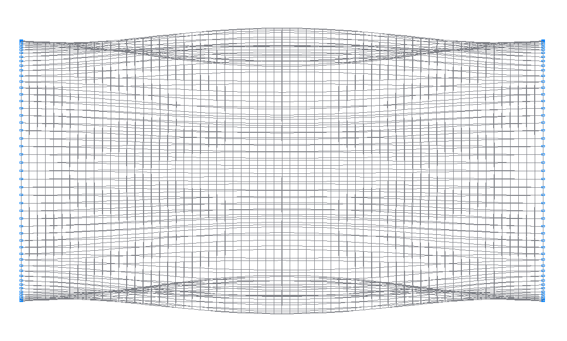
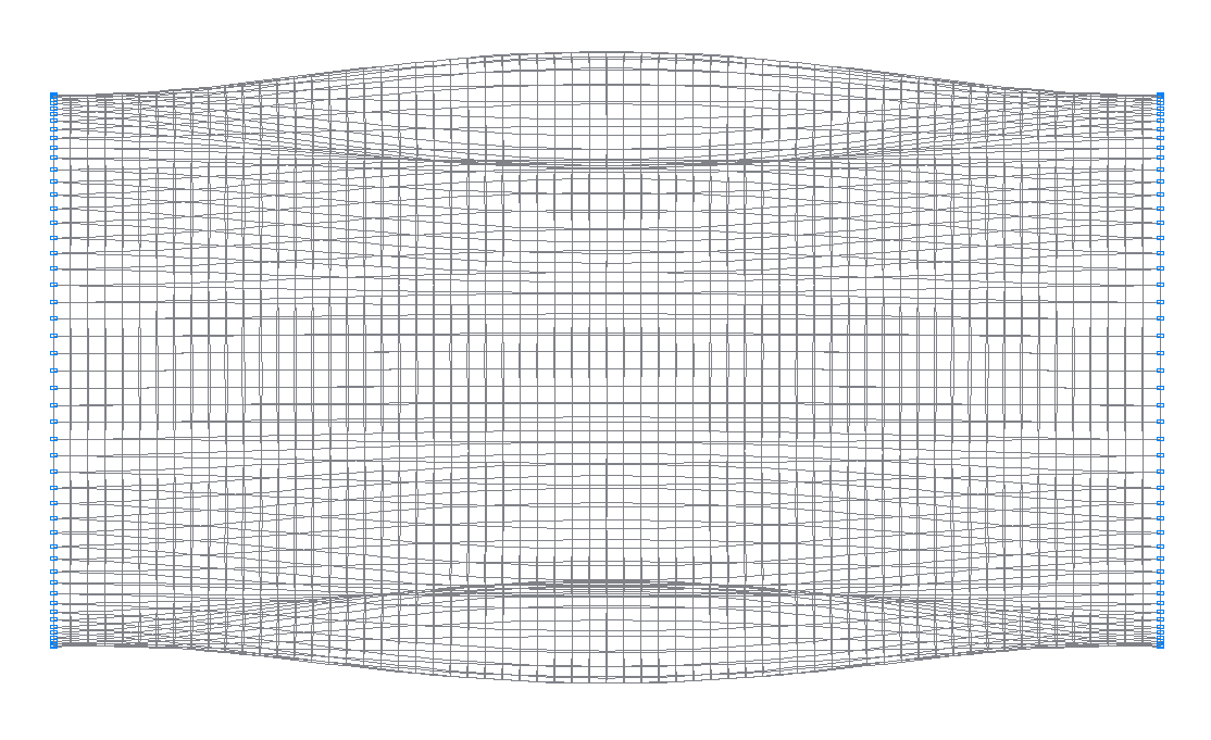
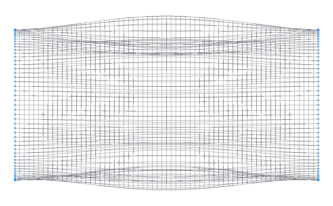
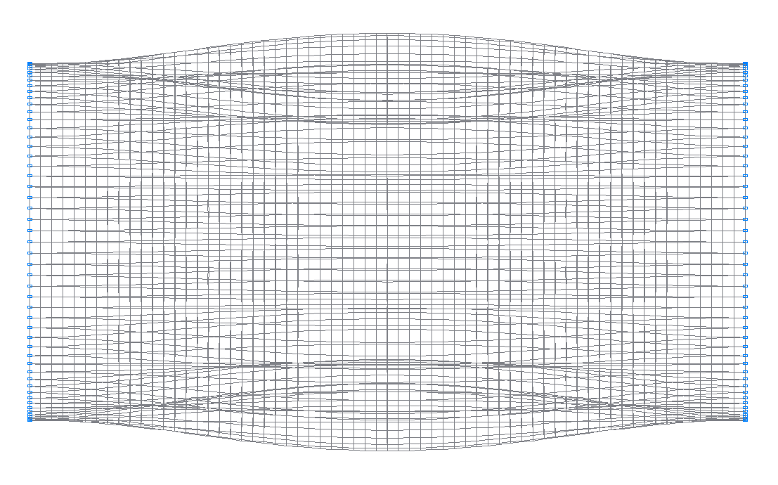
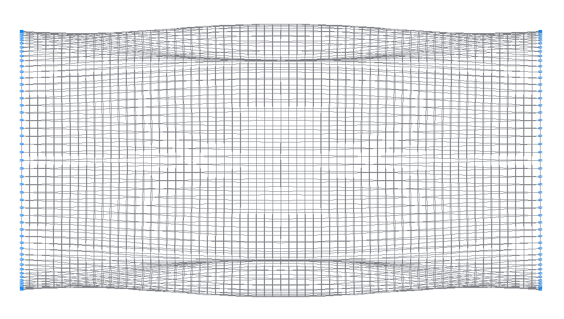
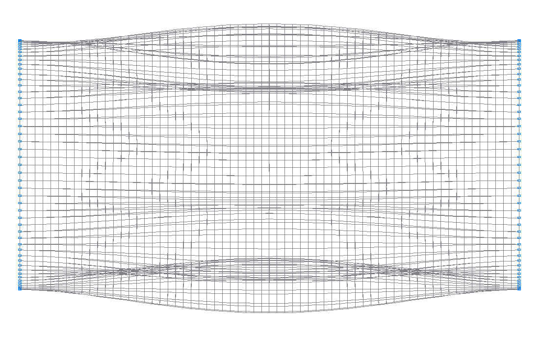
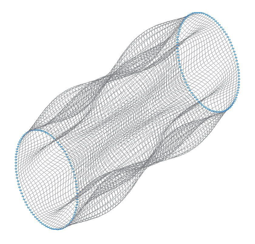
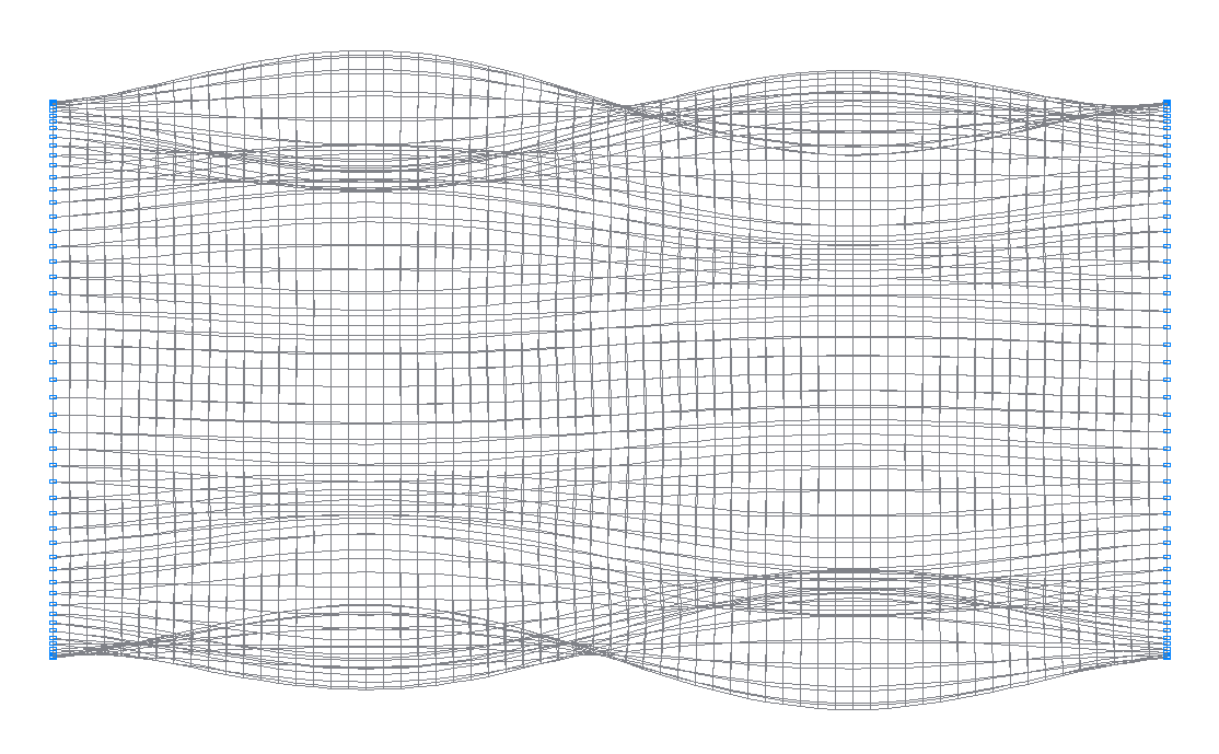
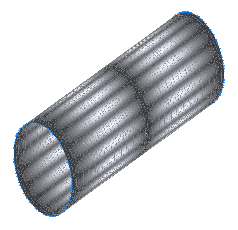
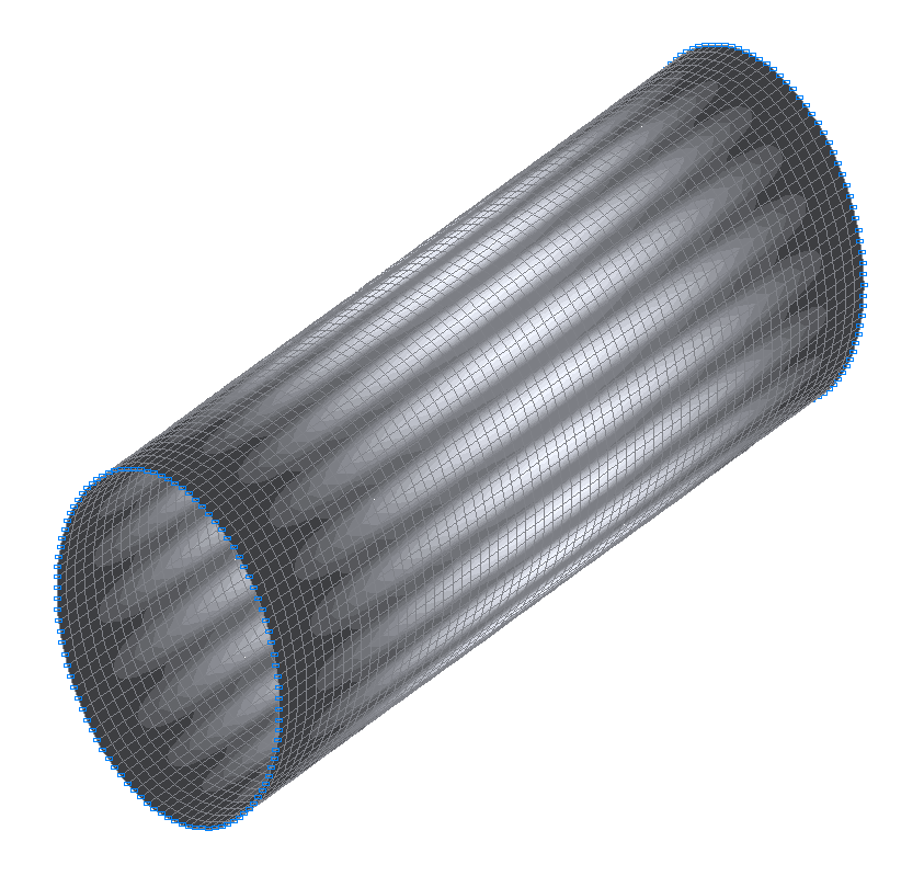
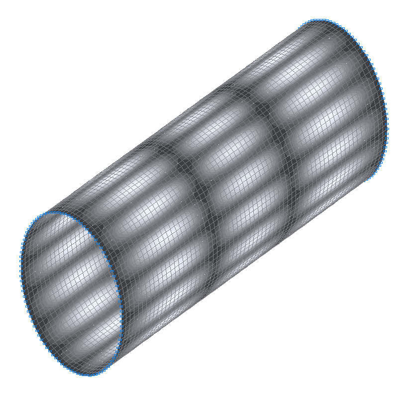
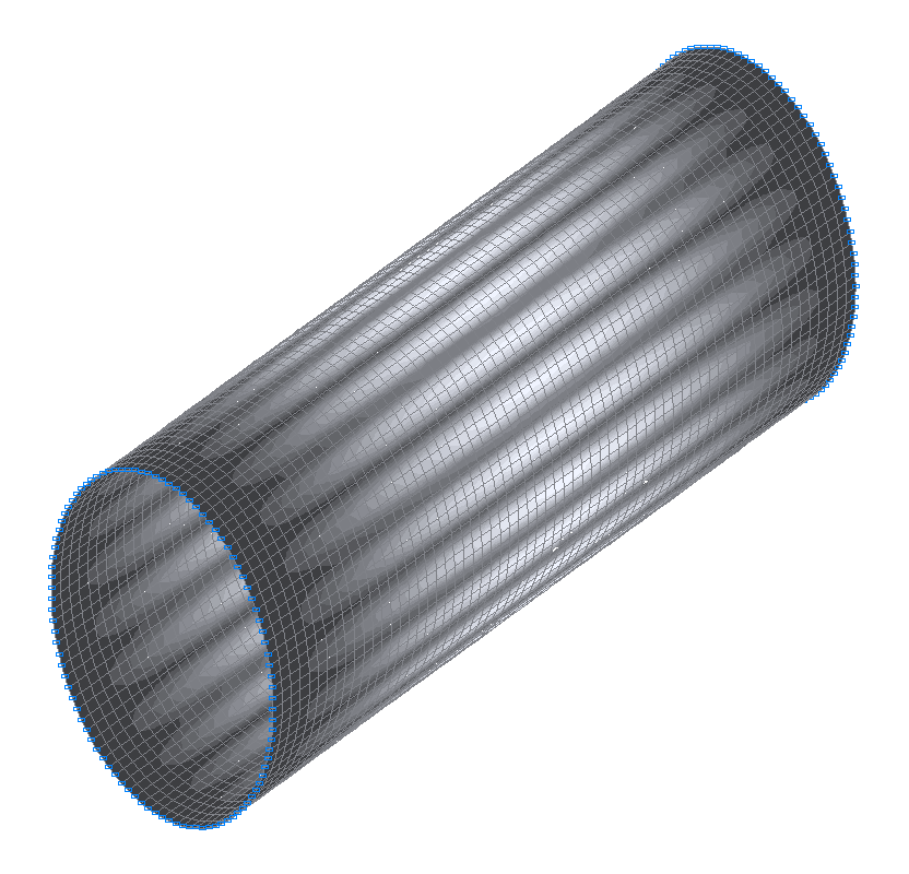
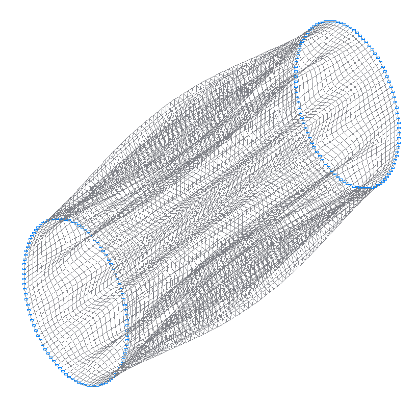
Finite element model: Design model – general type system, 6400 four-node shell elements of type 50. The spacing of the finite element mesh in the meridian direction is 4.765625·10-3 m (64 elements) and in the circumferential is 3.6º (100 elements). Boundary conditions of the simply supported edges are provided by imposing constraints in the directions of all linear and angular displacements (degrees of freedom X, Y, Z, UX, UY, UZ). The distributed mass is specified by transforming the static load from the self-weight of the cylindrical shell: ow = γ∙h, where γ = ρ∙g = 75.537 kN/m3. Number of nodes in the design model – 6500. The determination of the natural oscillation modes and natural frequencies is performed by the method of subspace iteration. The matrix of concentrated masses is used in the calculation.
Results in SCAD
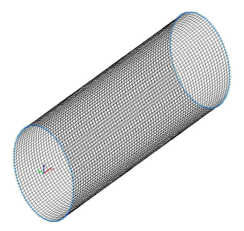
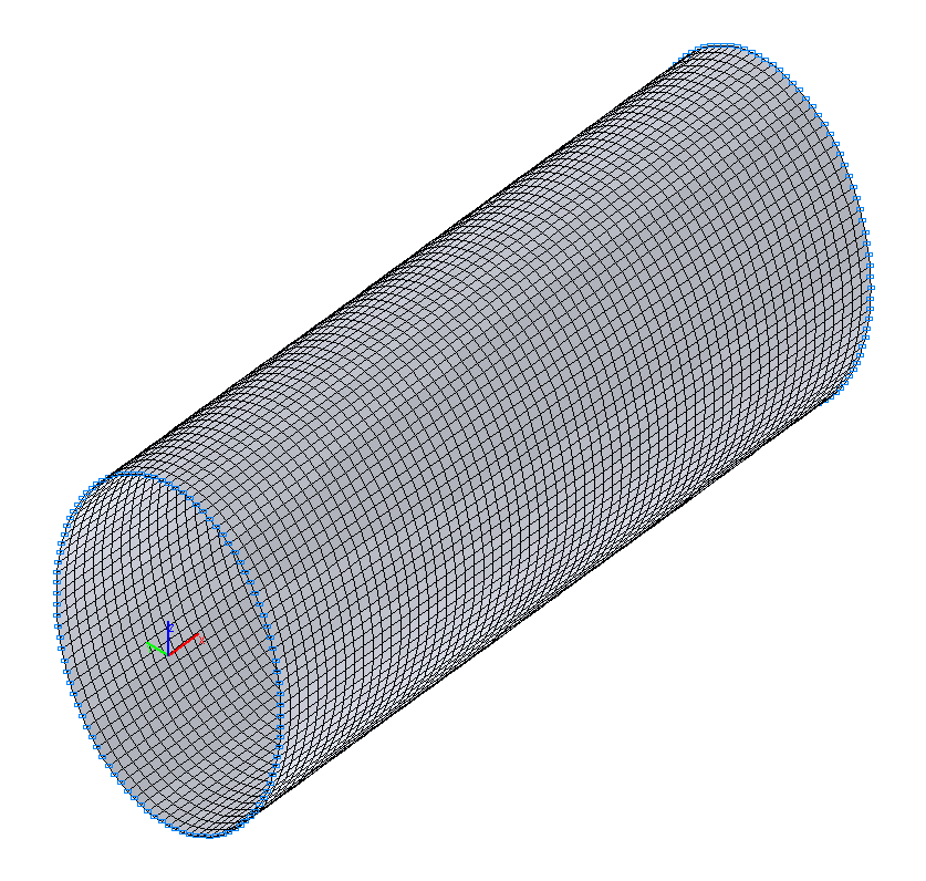
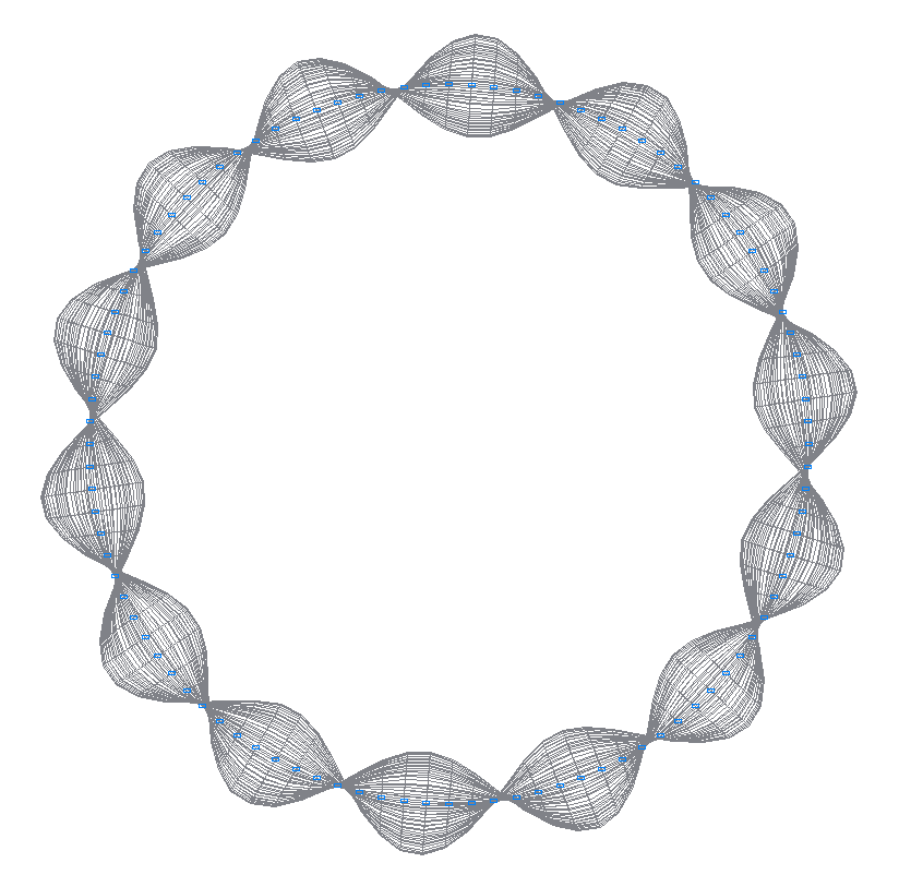
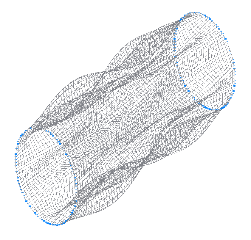
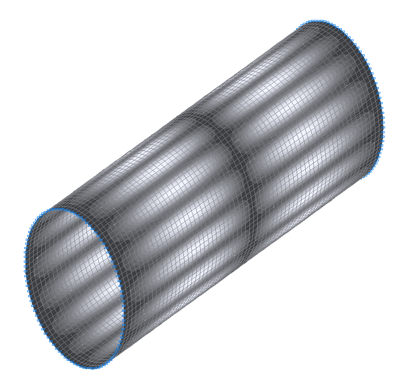
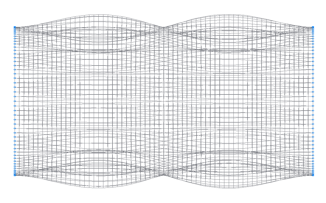
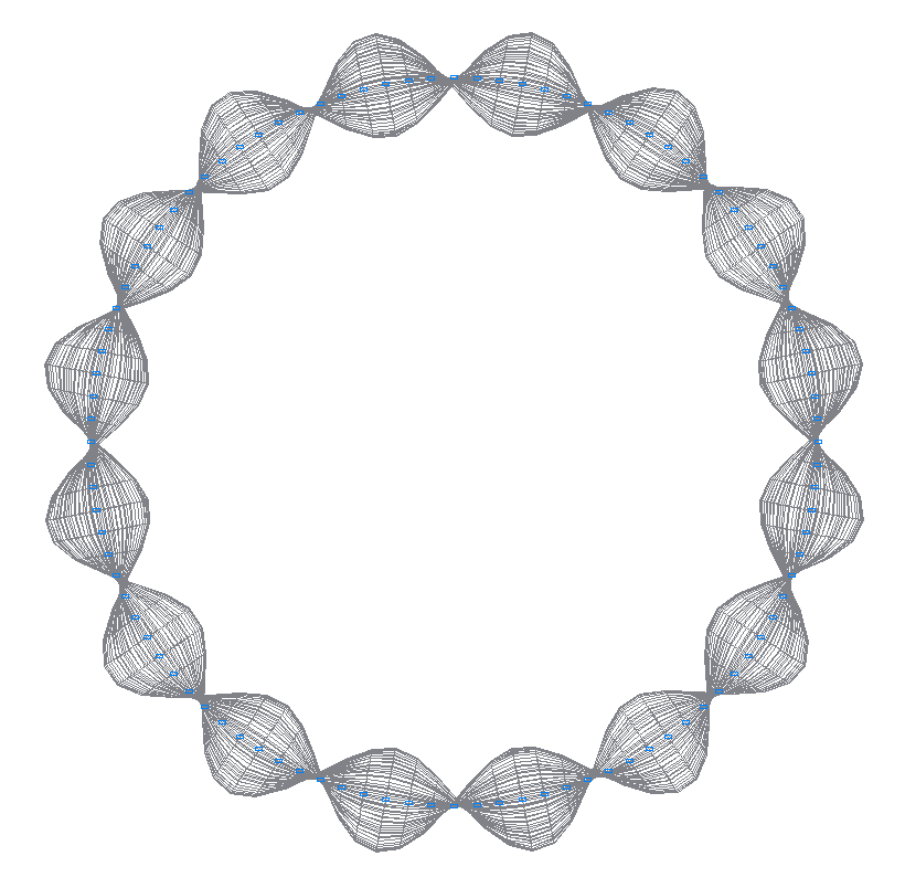
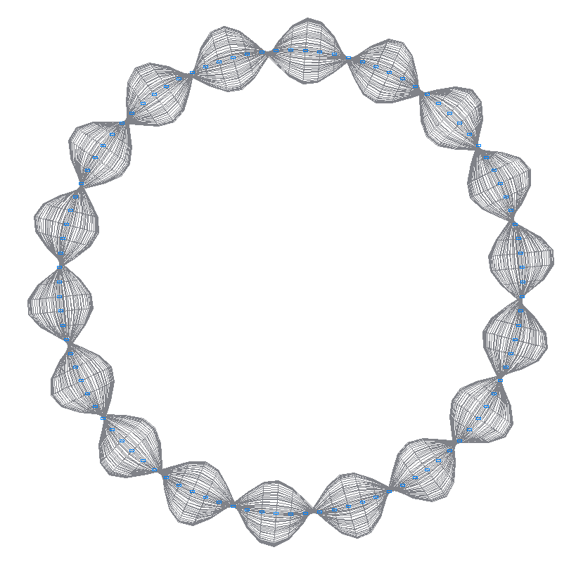
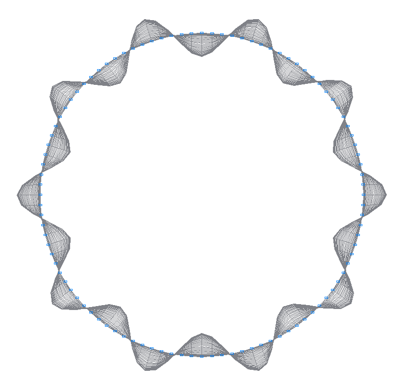
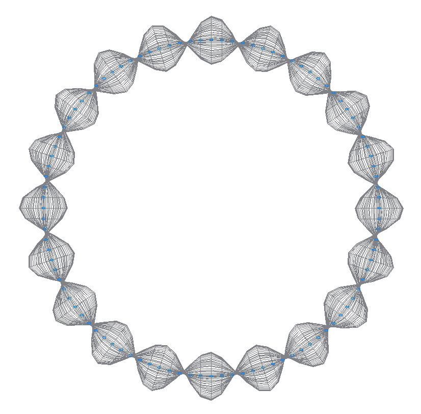
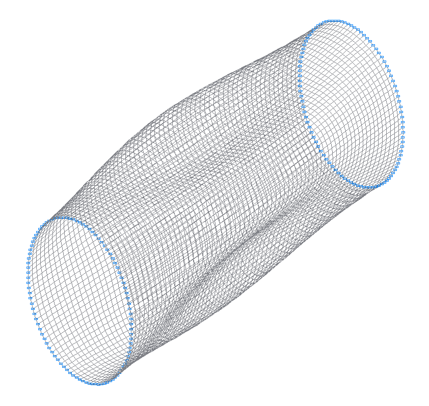
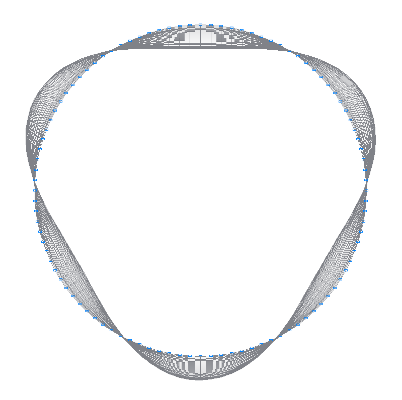
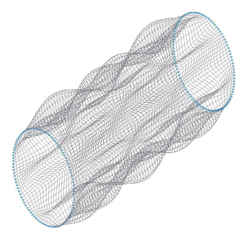
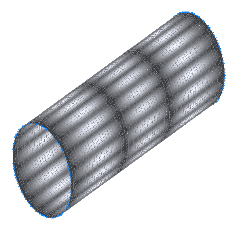
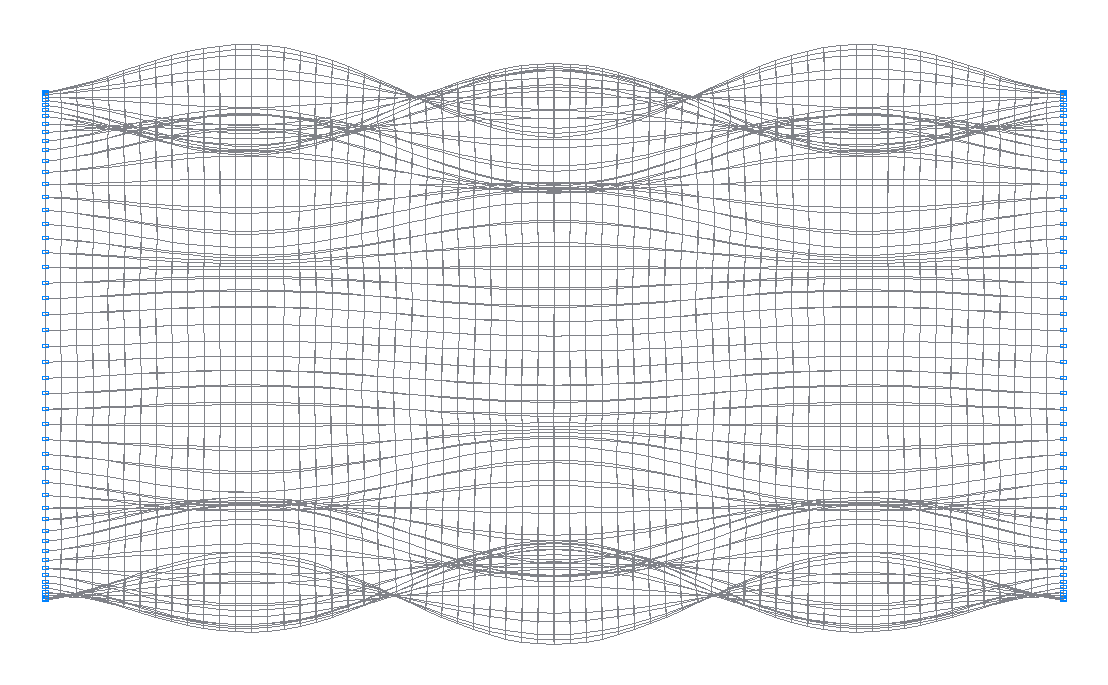
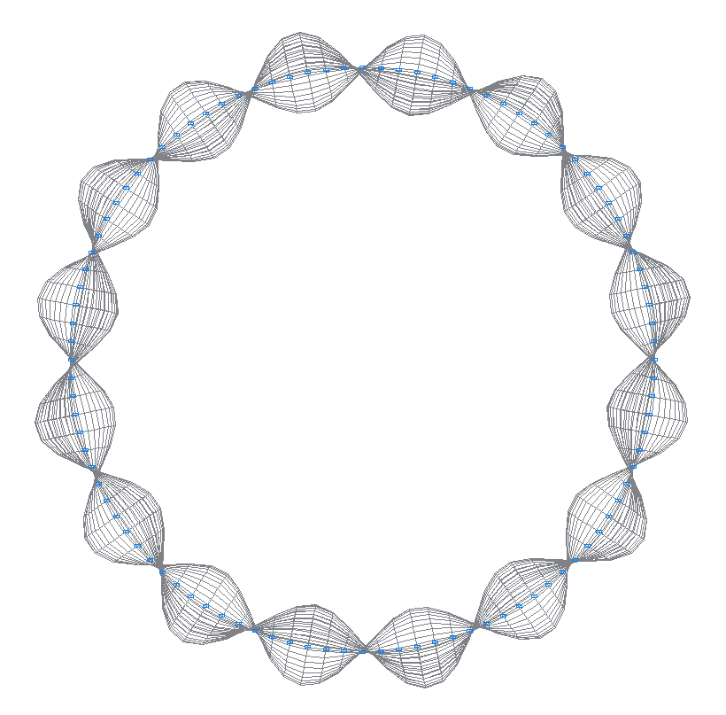
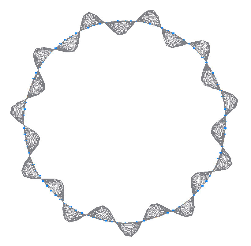
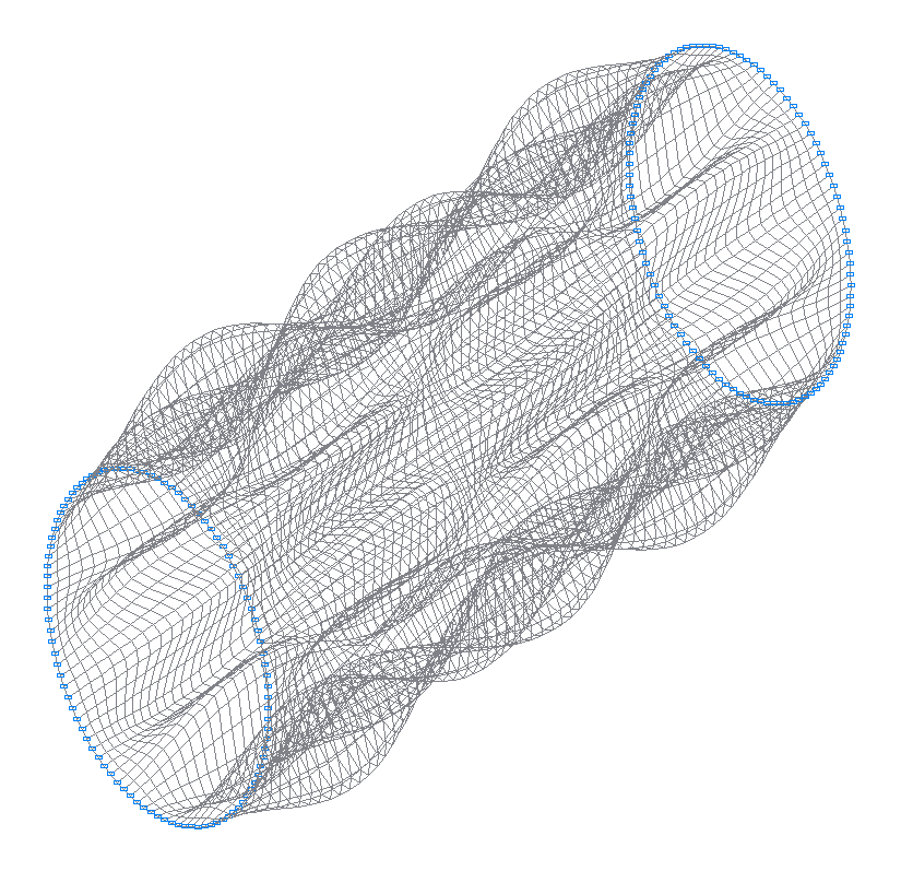
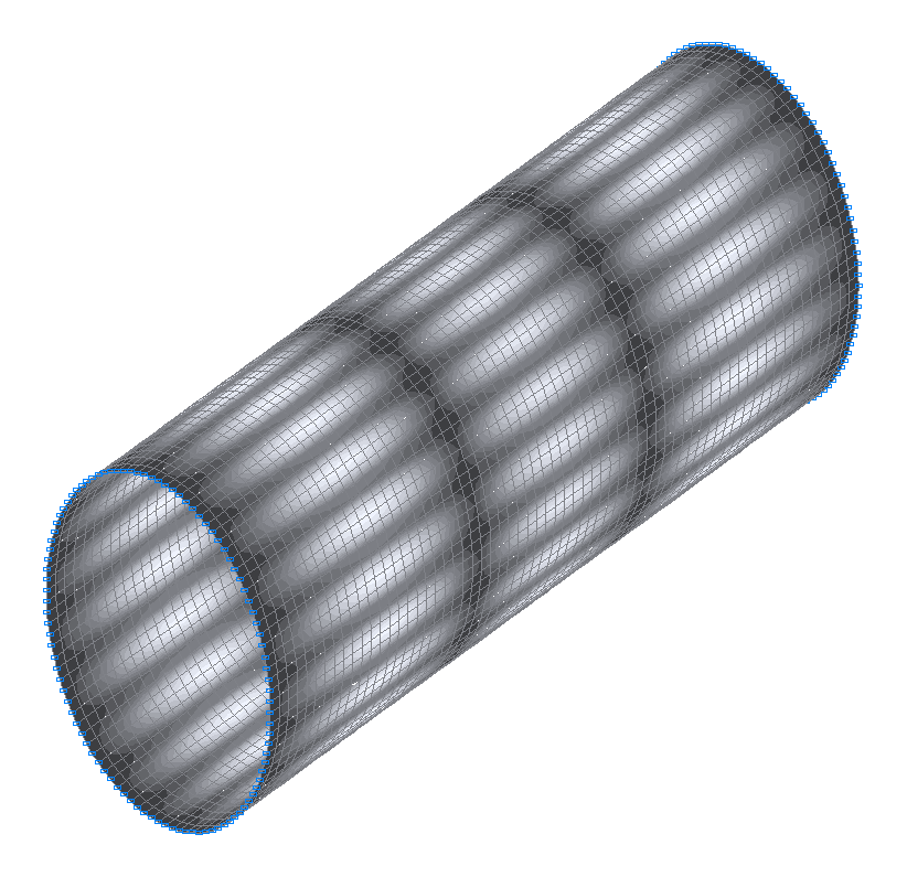
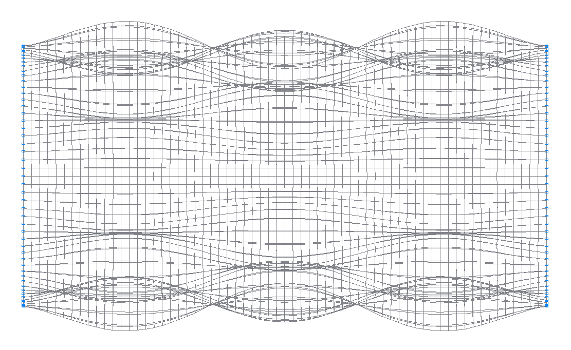
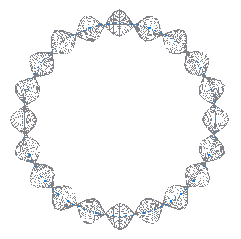
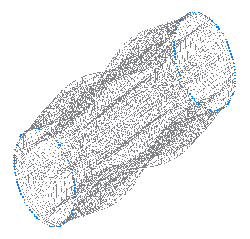
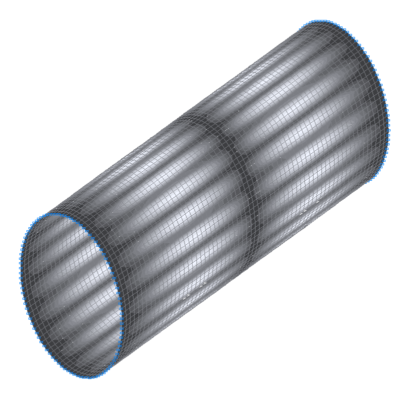
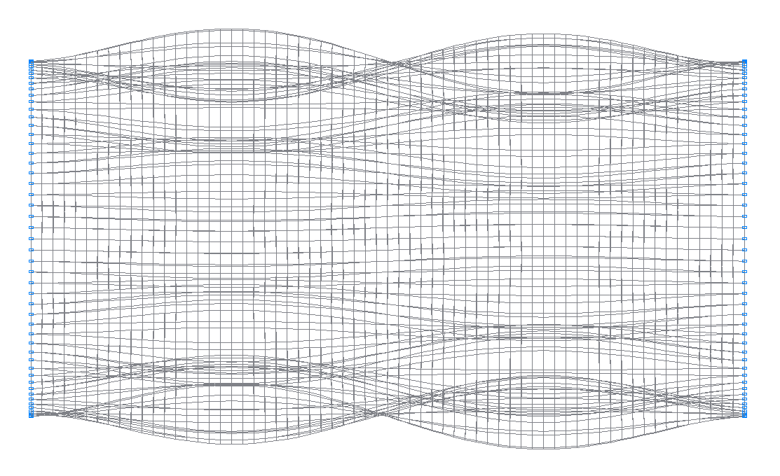
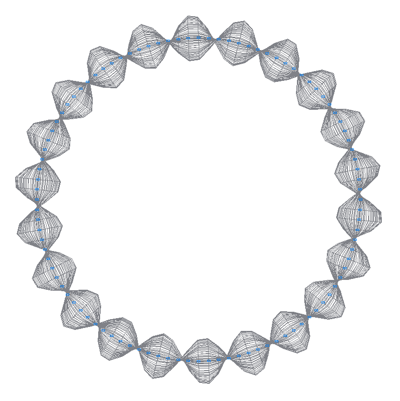
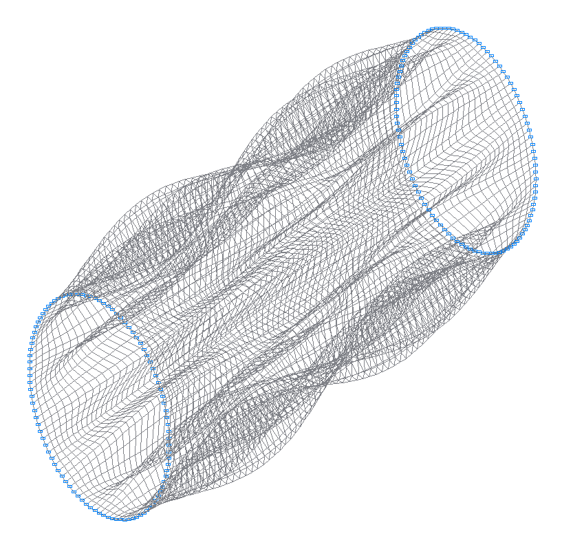
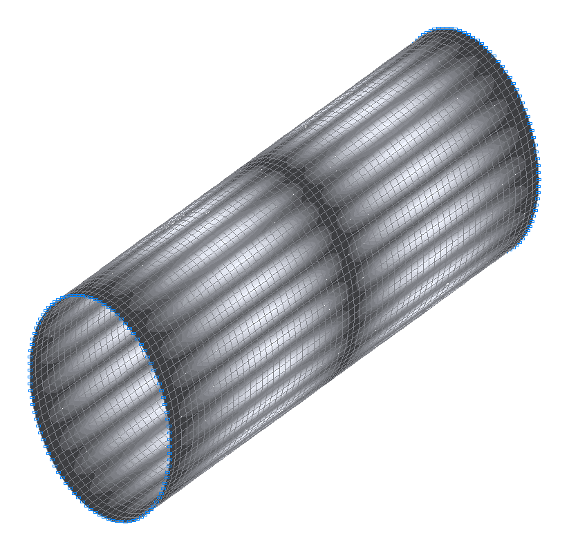
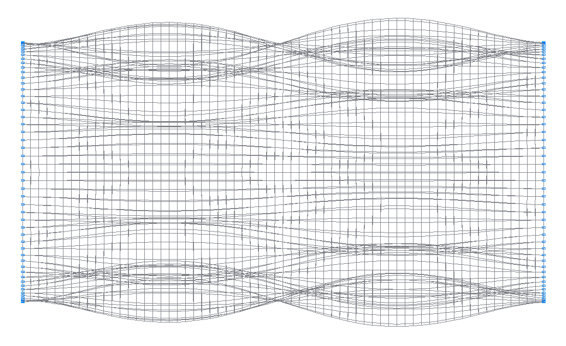
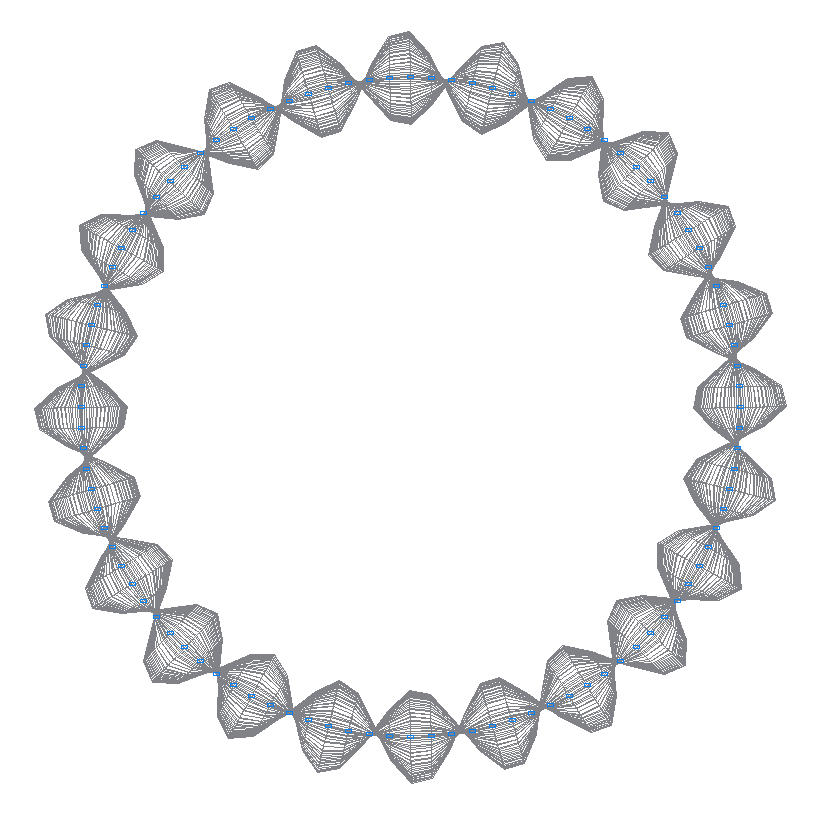
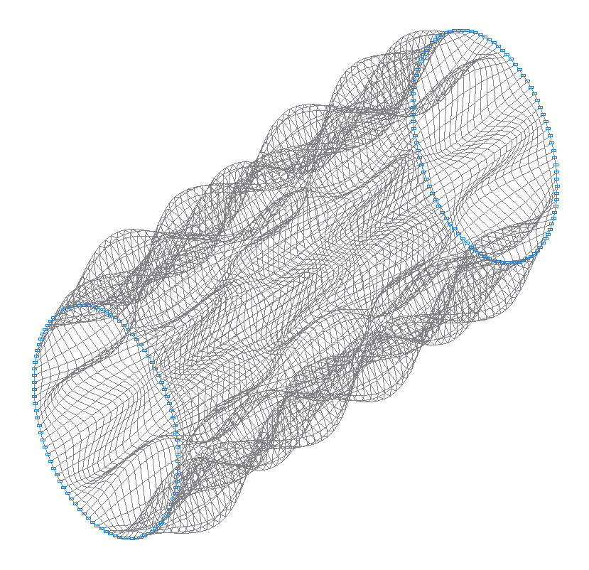
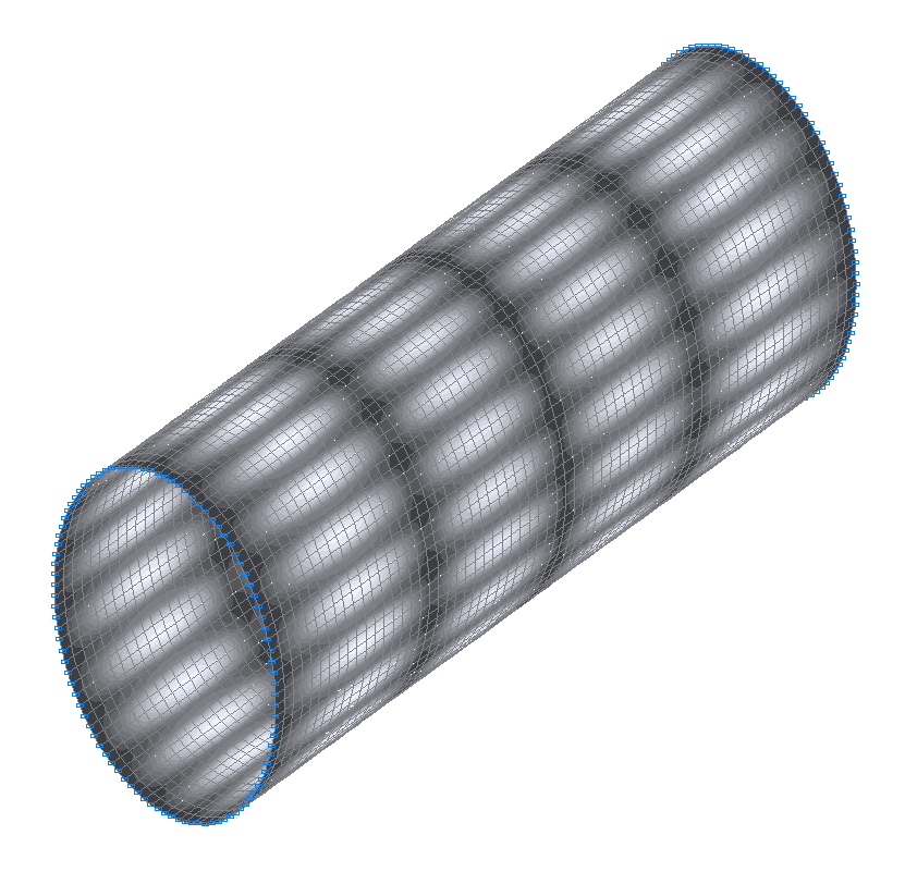
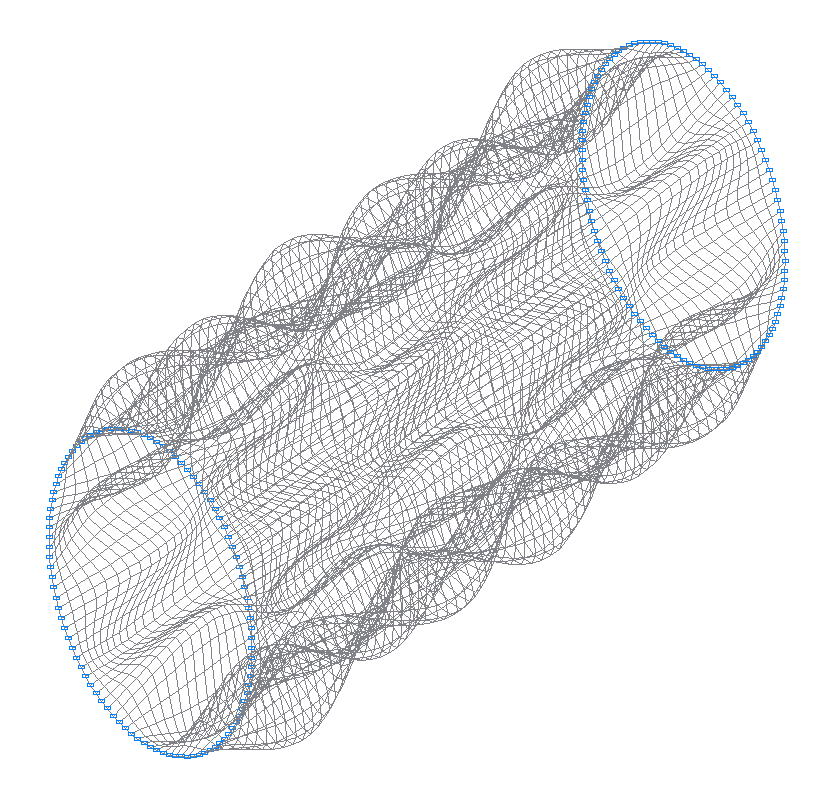
Design model
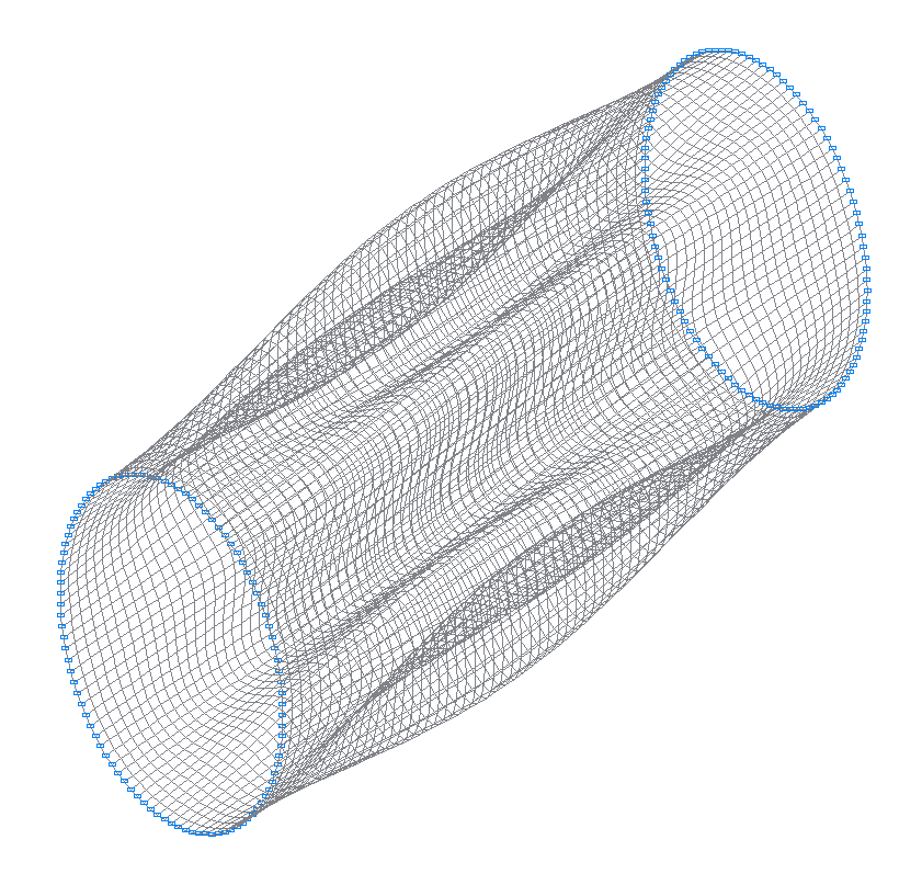
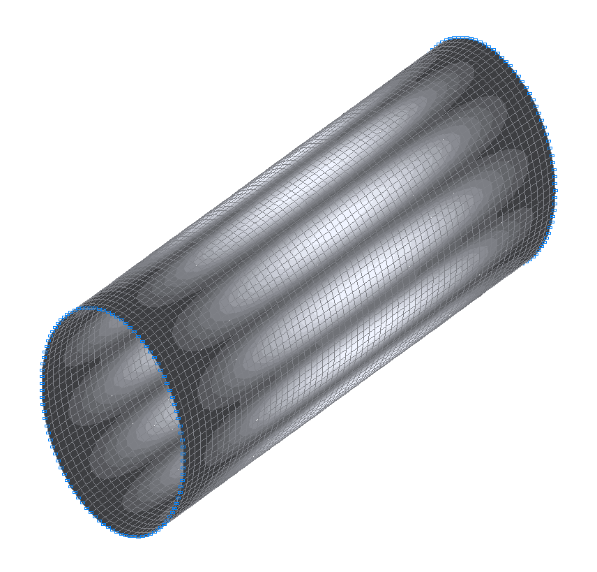
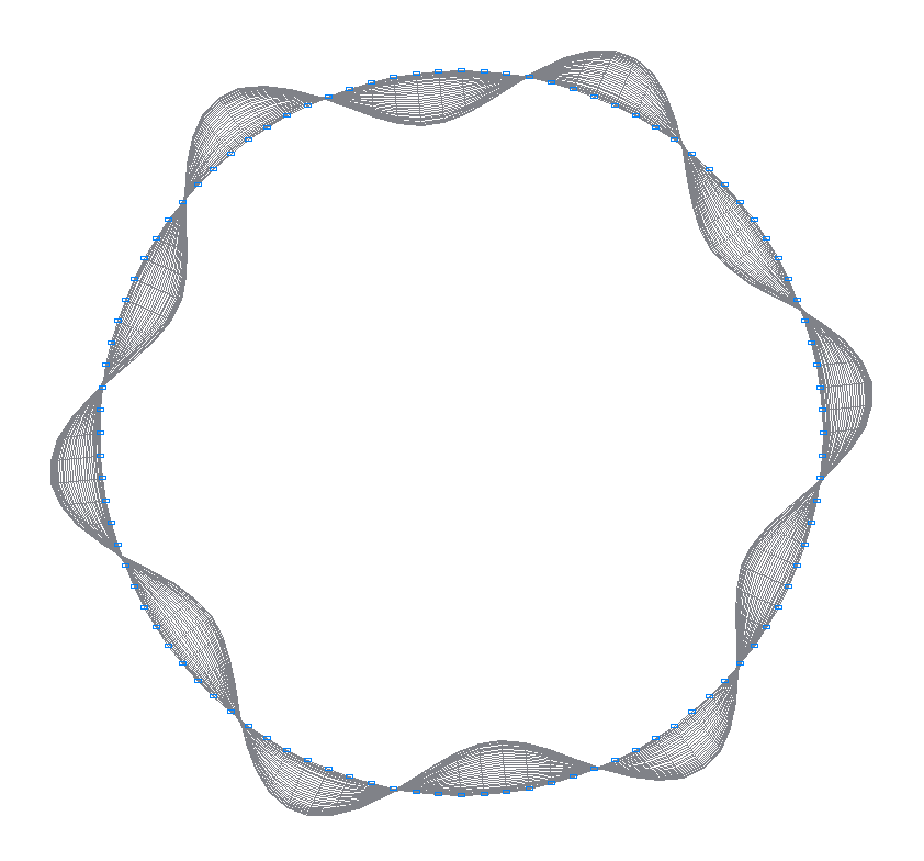
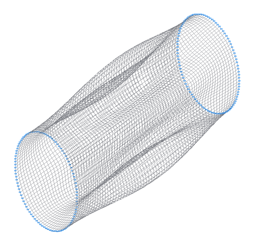
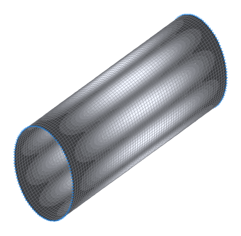
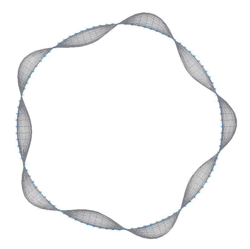
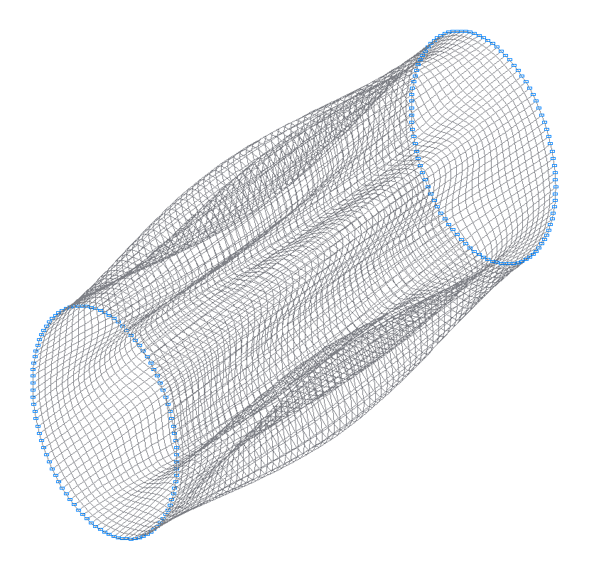
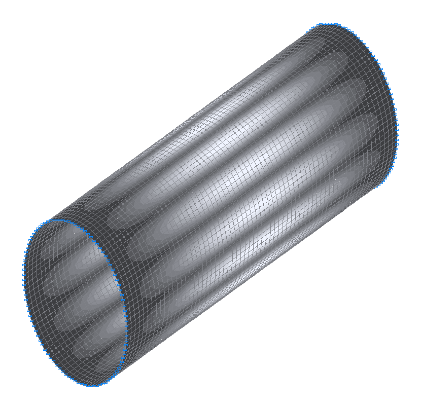
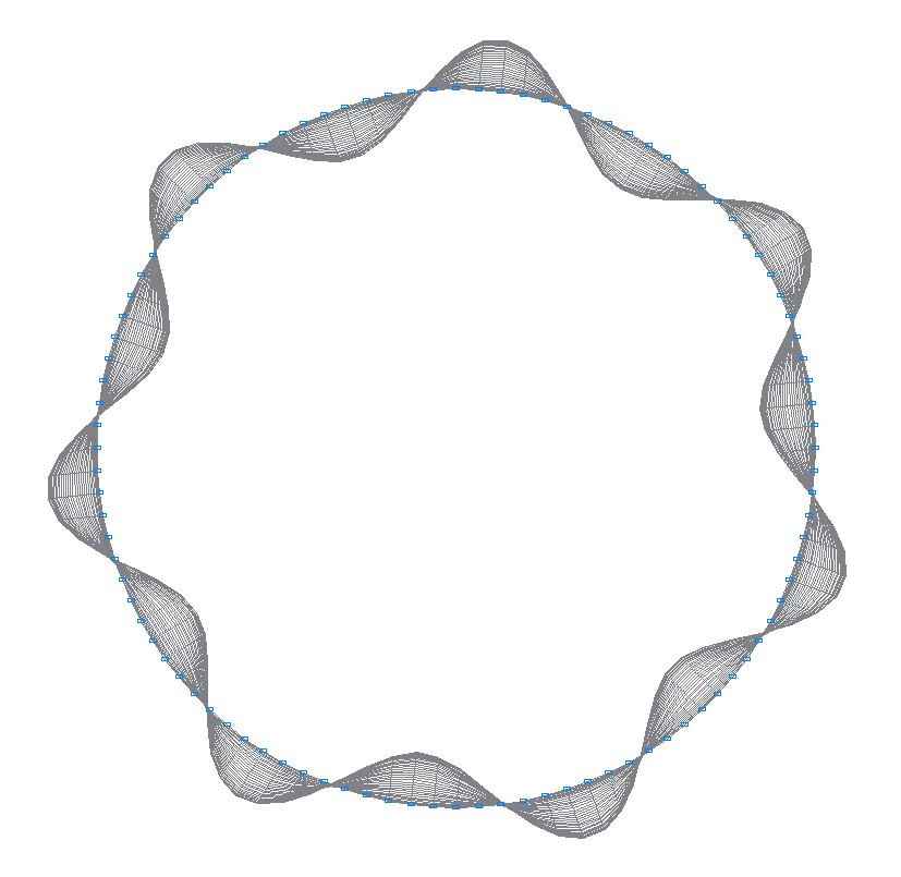
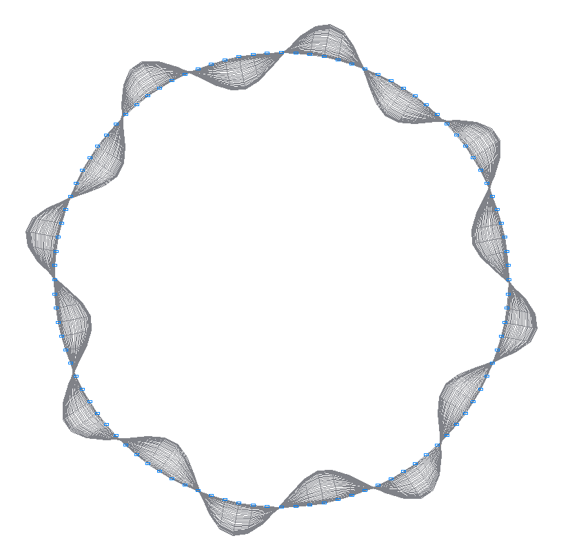
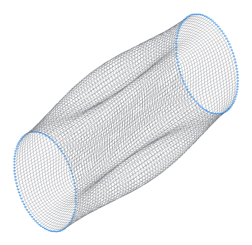
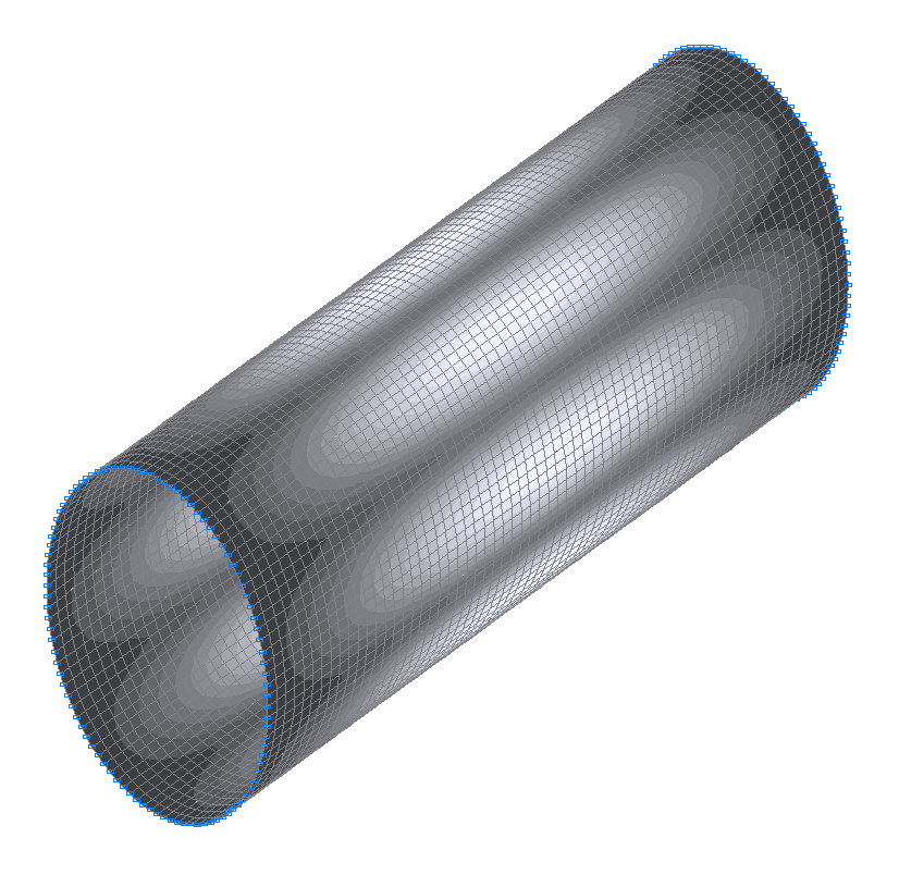
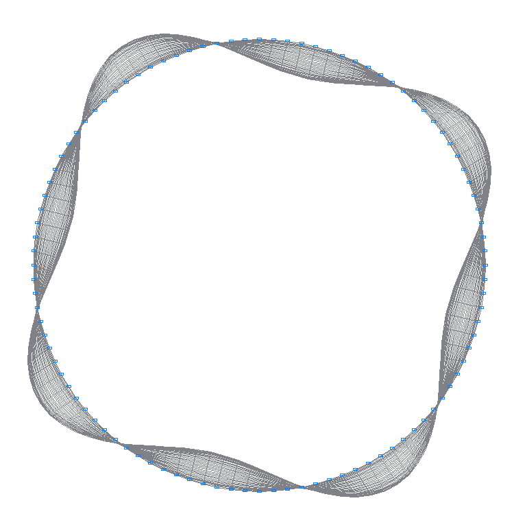
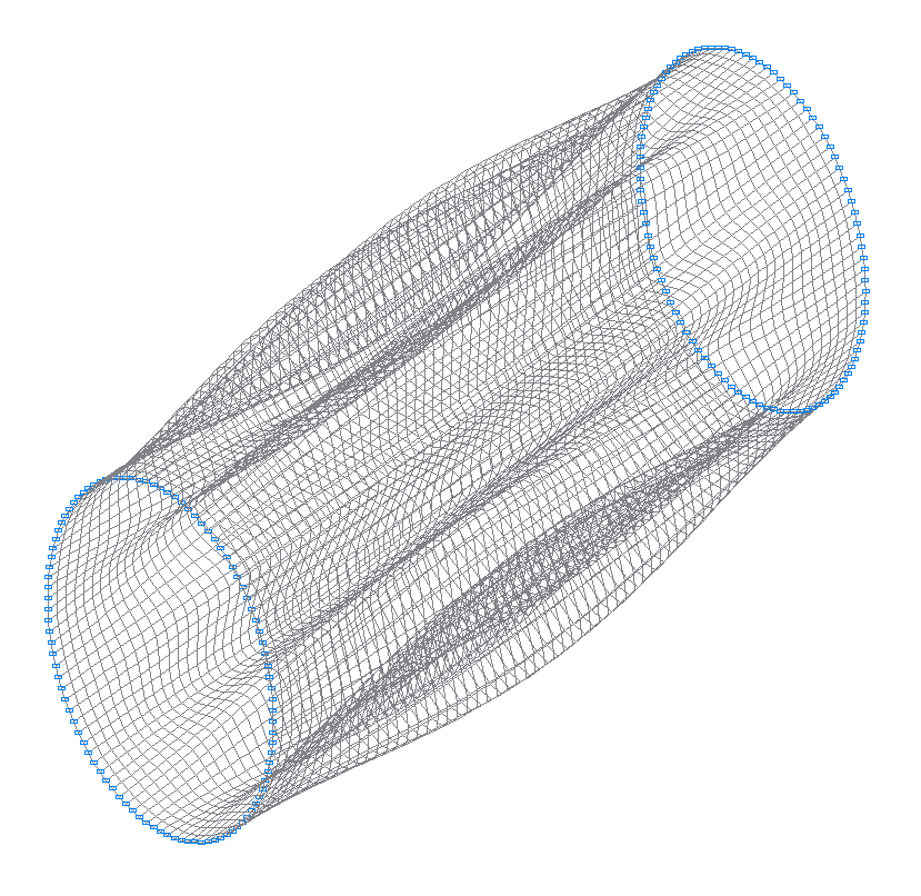
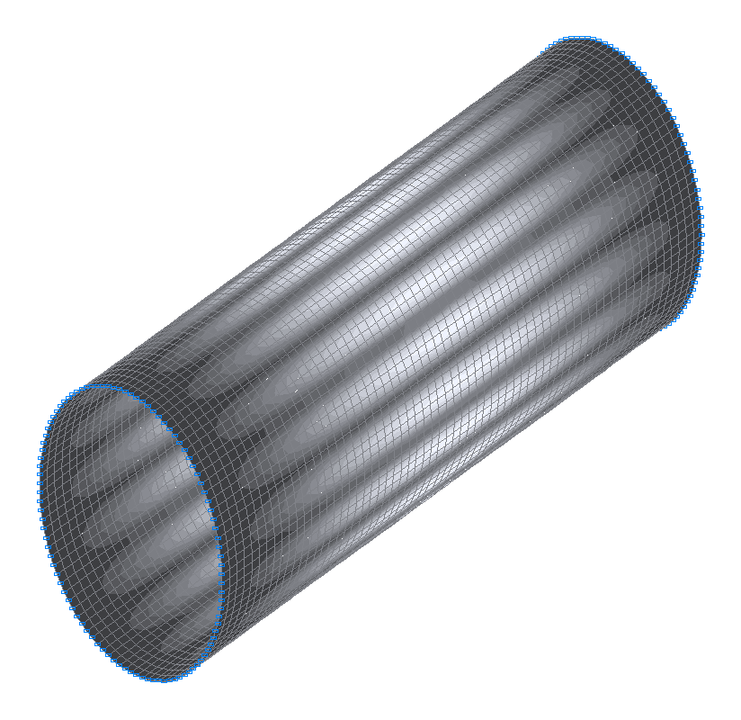
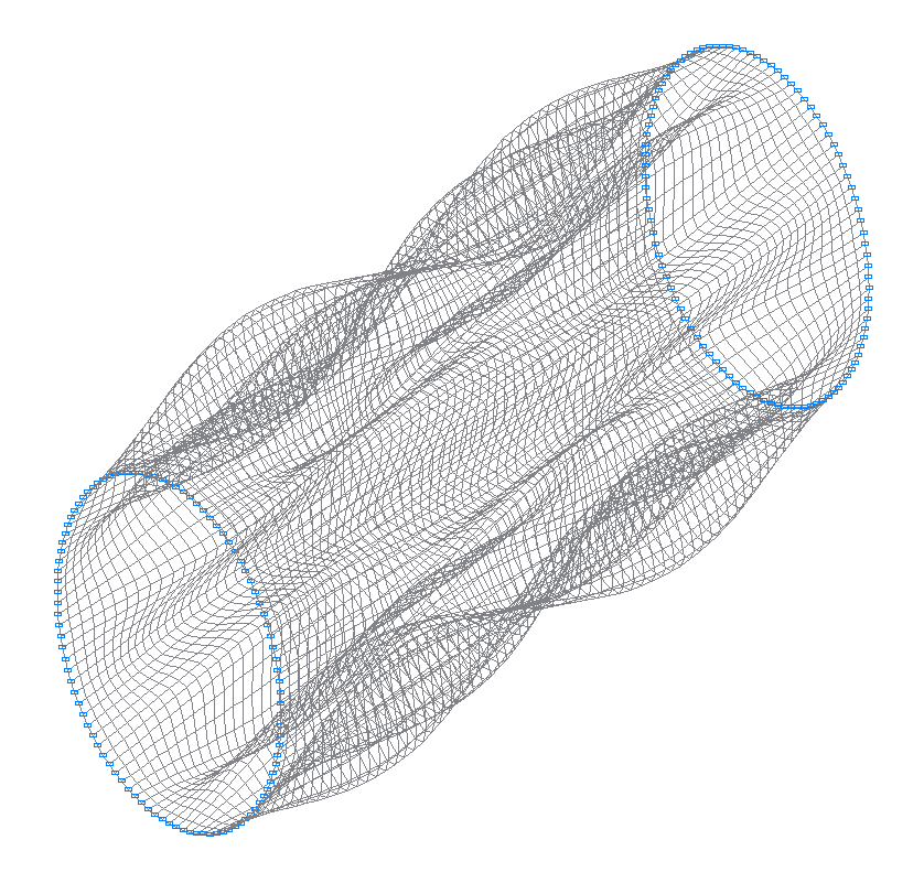
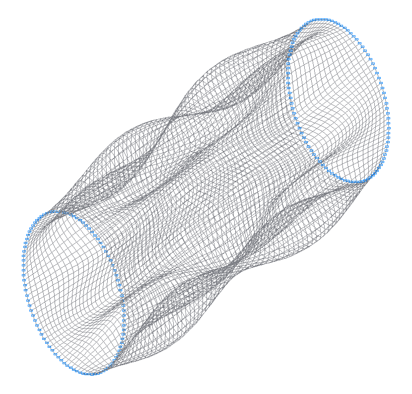
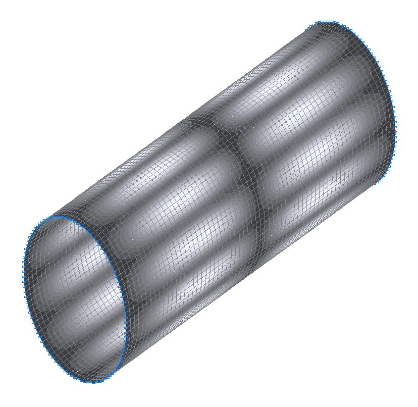
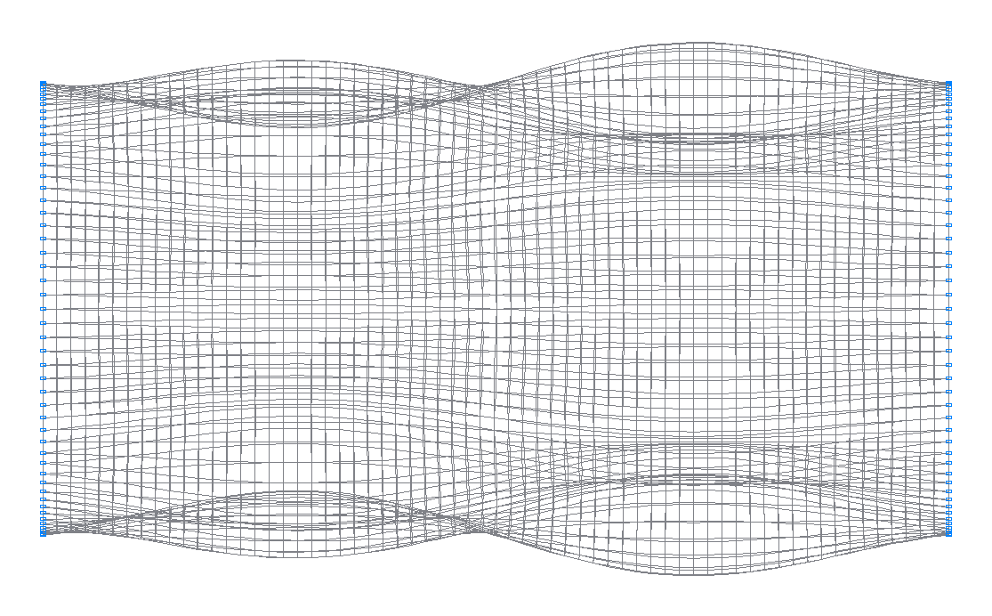
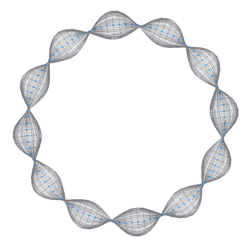
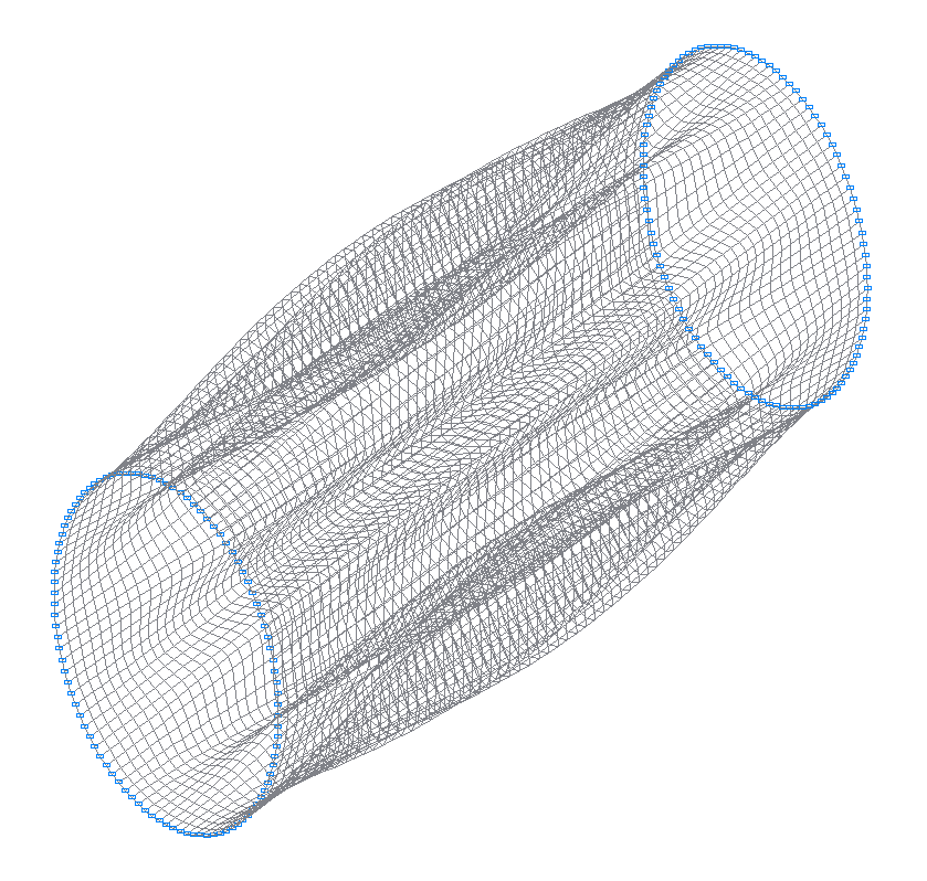
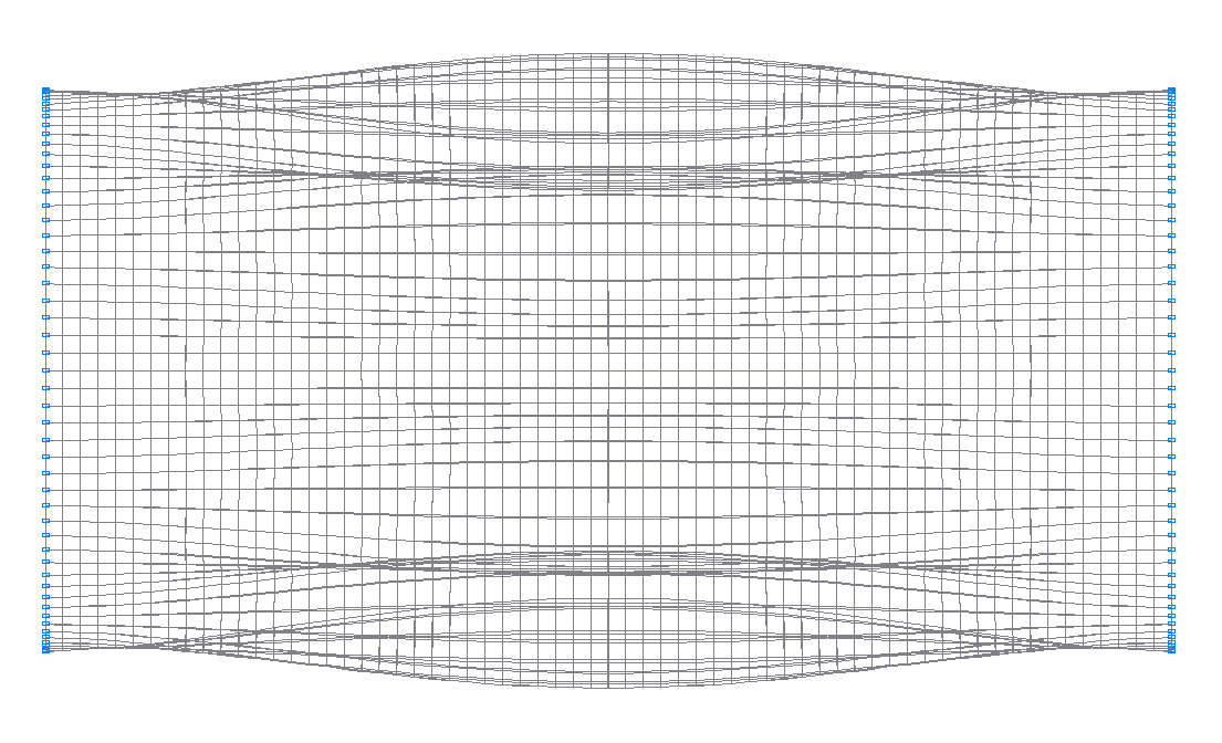
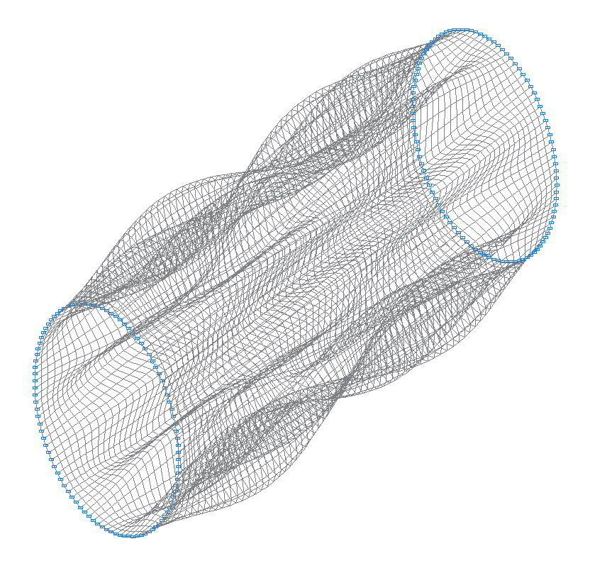
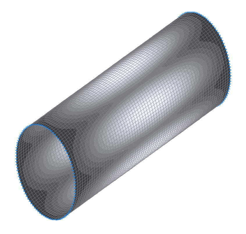
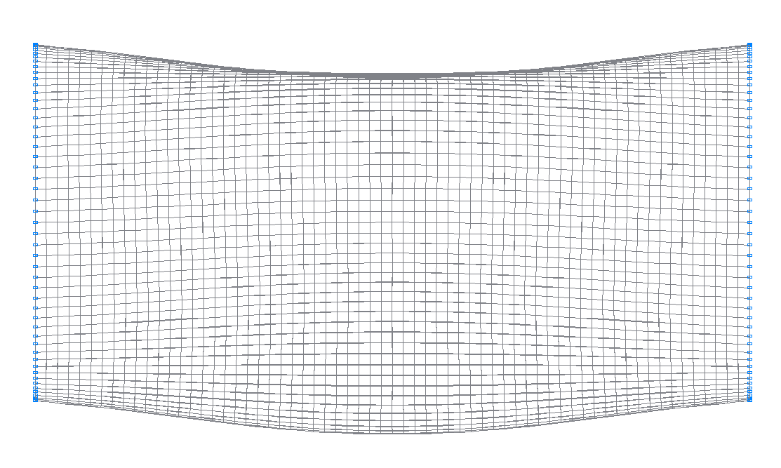
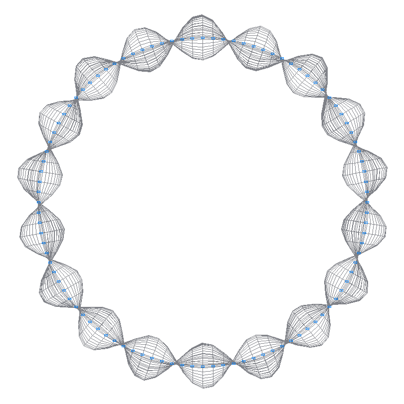
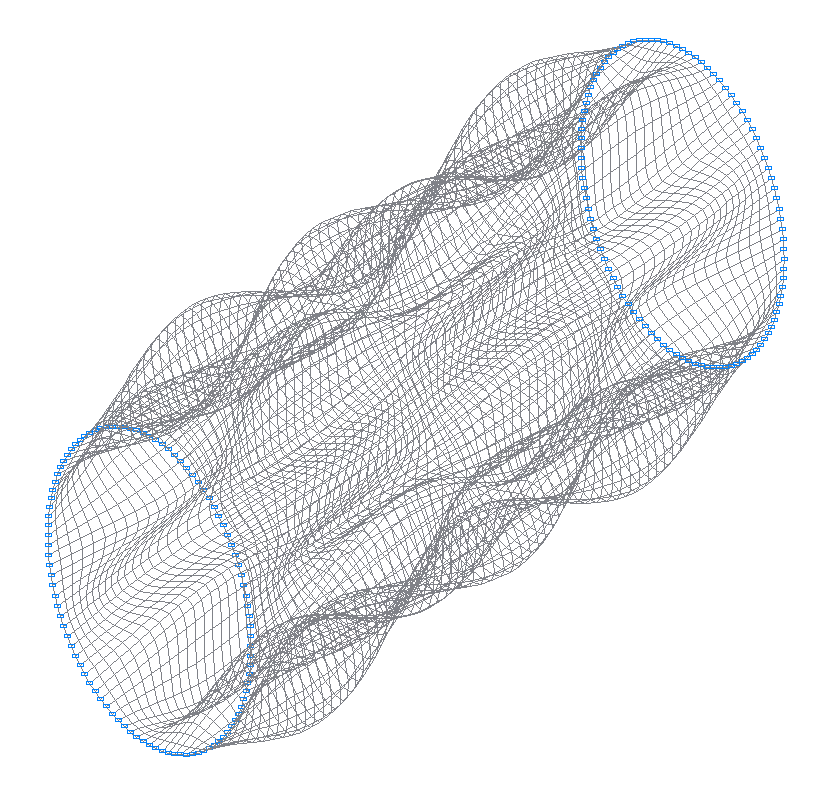
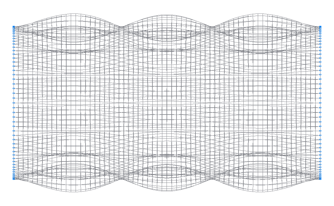
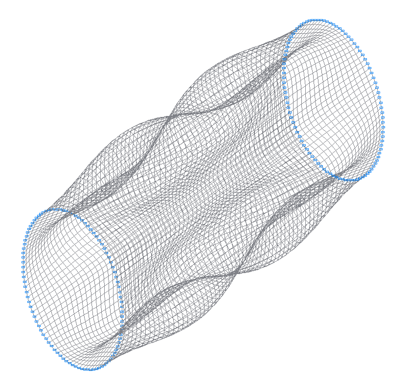
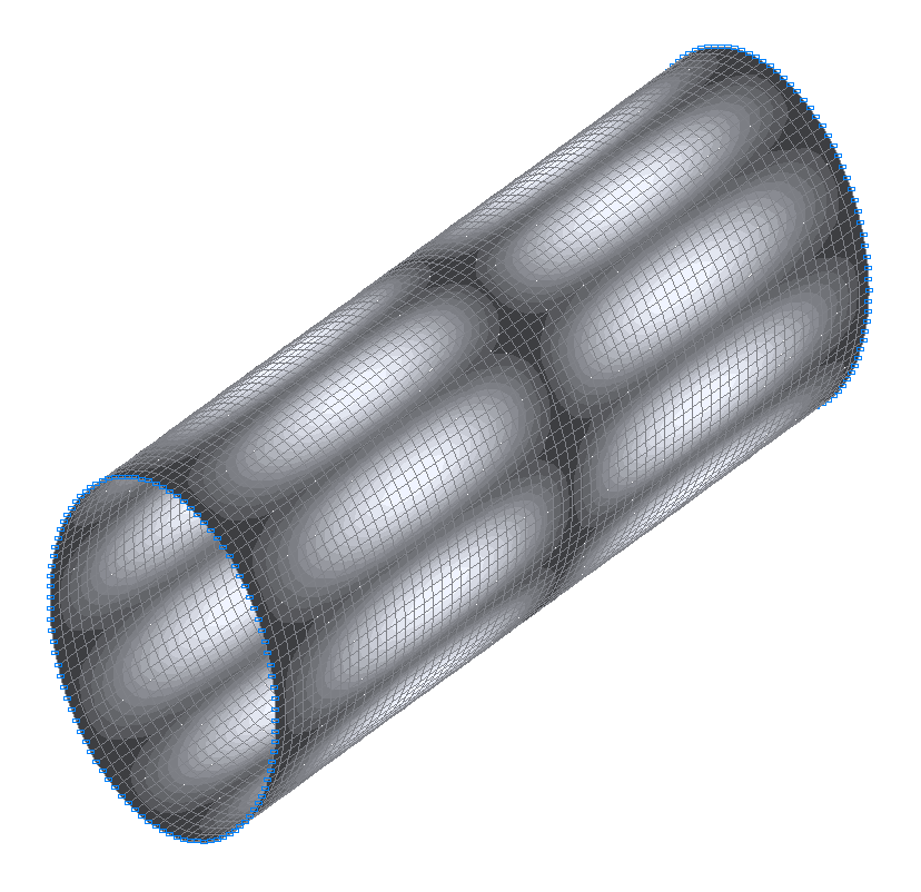
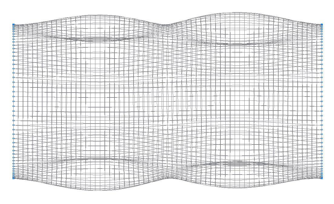
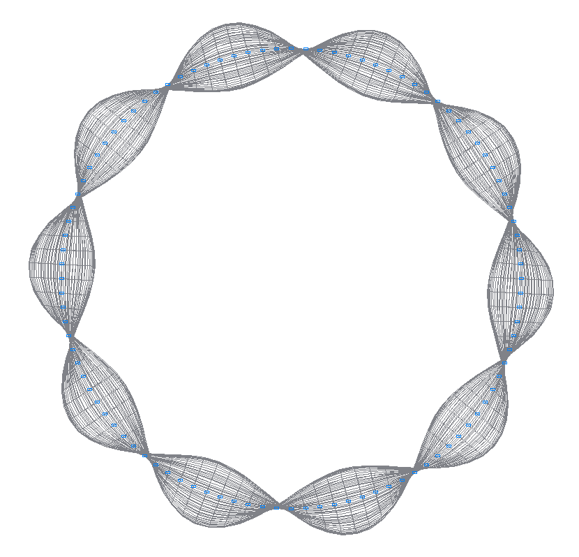
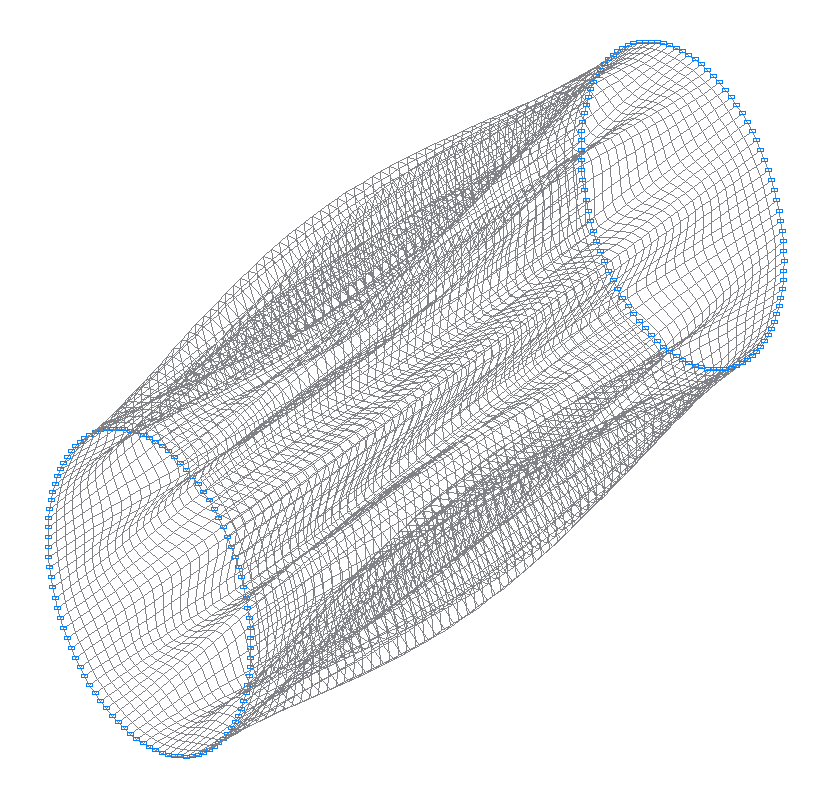
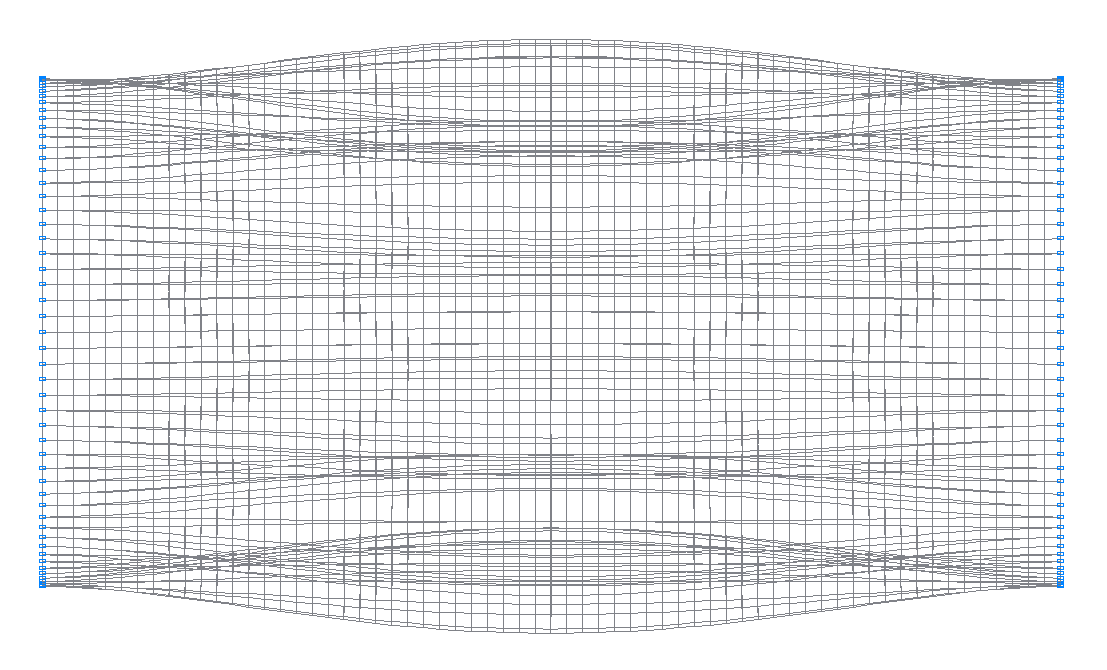
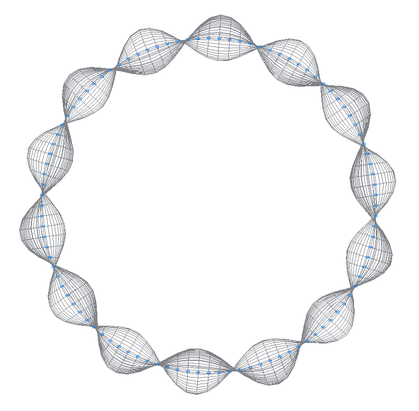
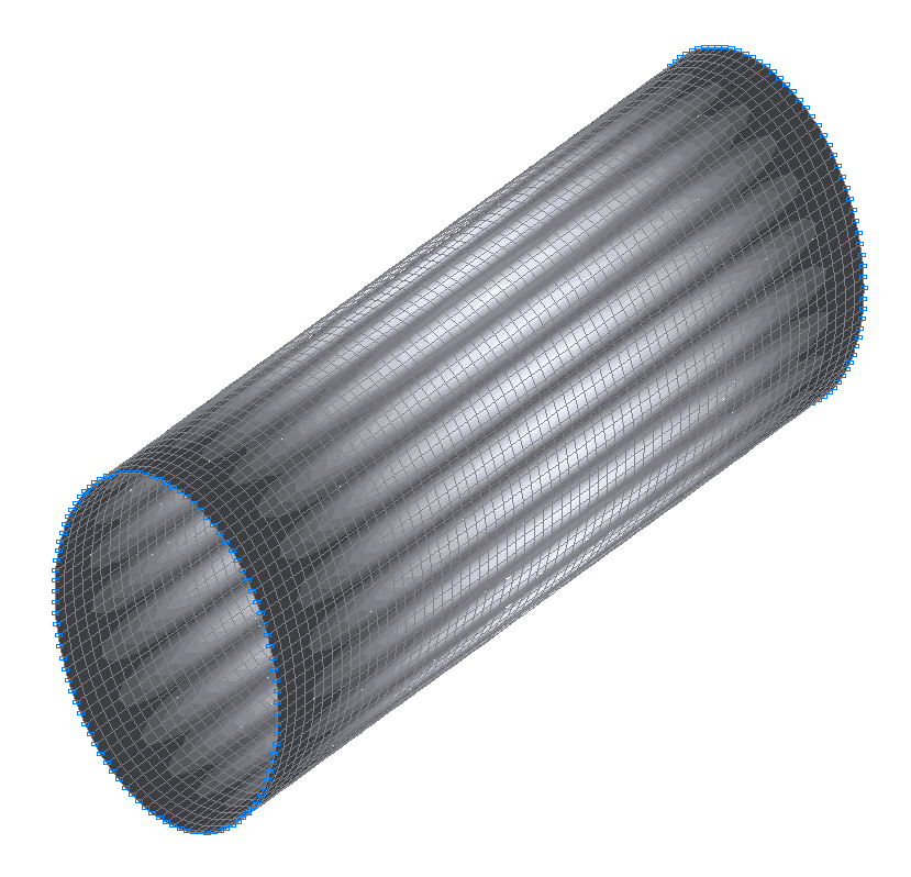
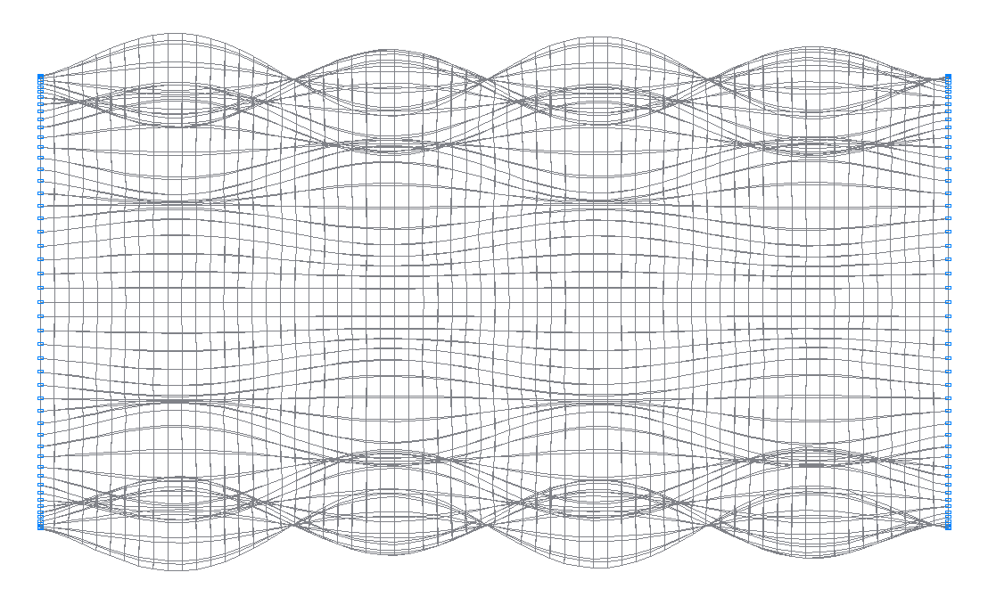
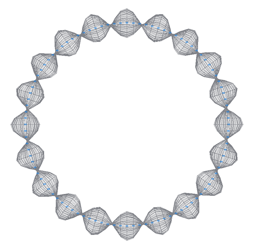
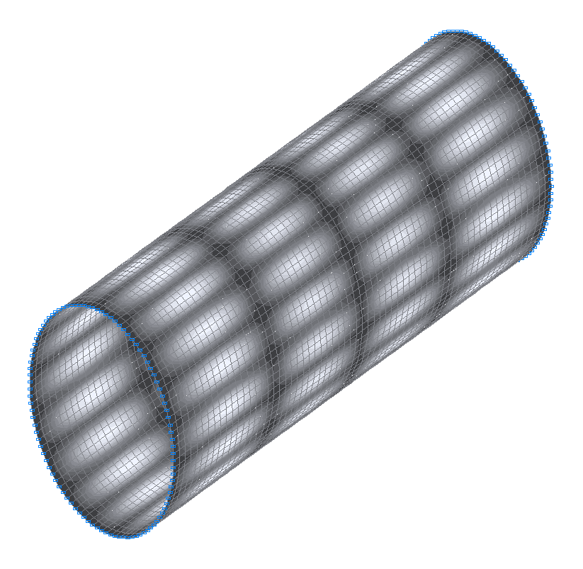
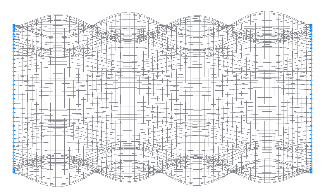
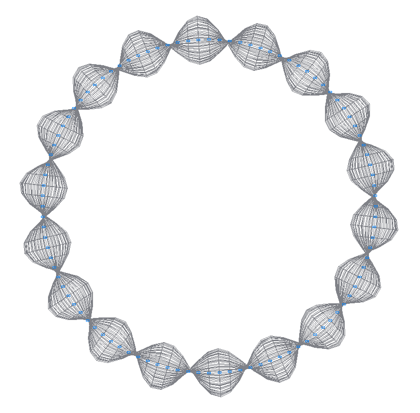
1-st (1-st theoretical) natural oscillation mode
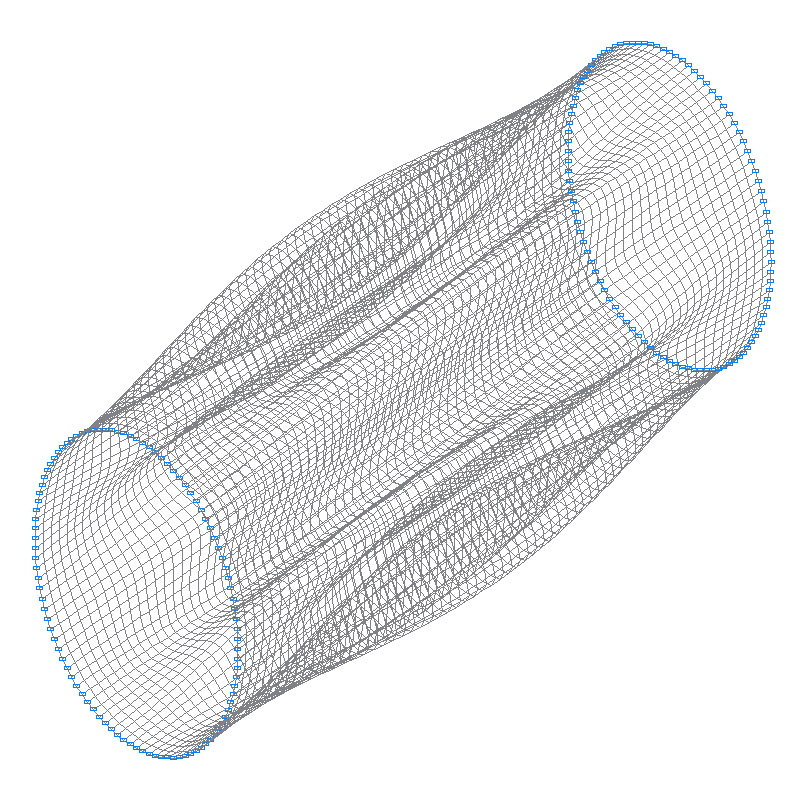
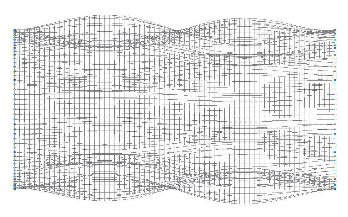
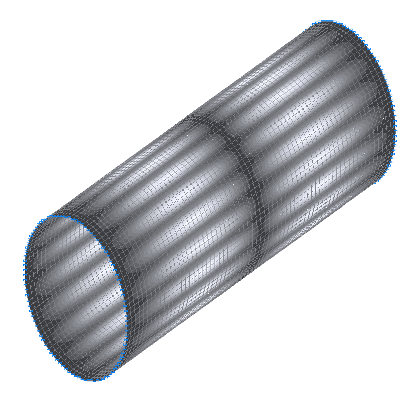
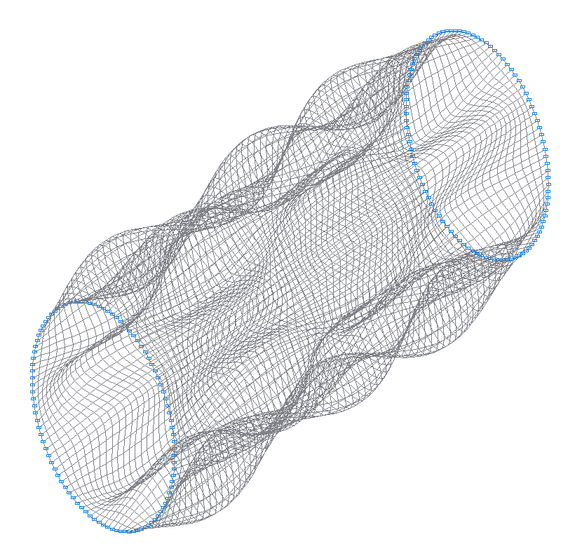
3-rd (3-rd theoretical) natural oscillation mode
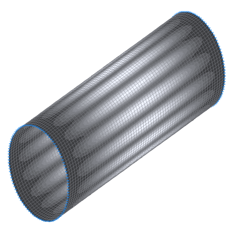
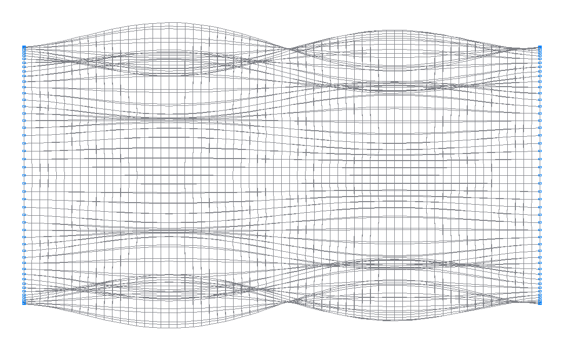
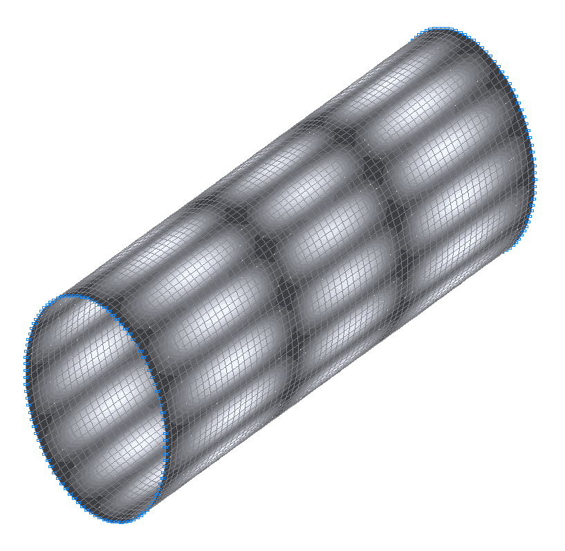
5-th (5-th theoretical) natural oscillation mode
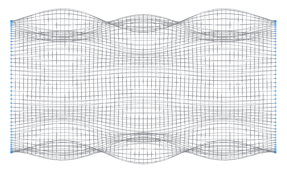
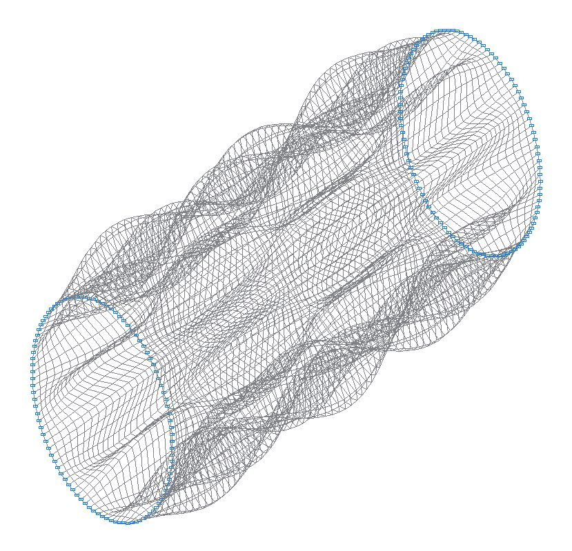
7-th (7-th theoretical) natural oscillation mode
9-th (9-th theoretical) natural oscillation mode
11-th (11-th theoretical) natural oscillation mode

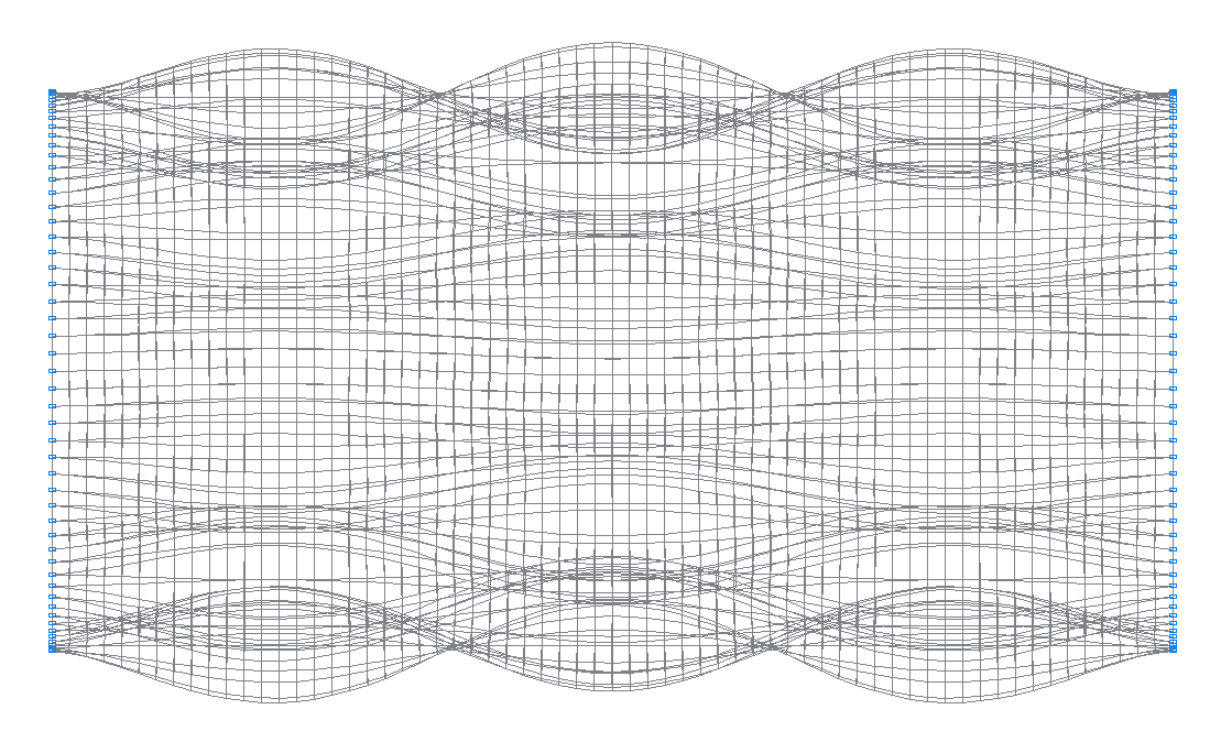
13-th (13-th theoretical) natural oscillation mode
15-th (15-th theoretical) natural oscillation mode
17-th (17-th theoretical) natural oscillation mode
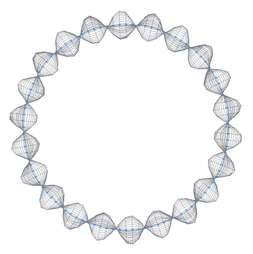
19-th (19-th theoretical) natural oscillation mode
21-st (21-st theoretical) natural oscillation mode
23-rd (25-th theoretical) natural oscillation mode
25-th (23-rd theoretical) natural oscillation mode
27-th (27-th theoretical) natural oscillation mode
29-th (31-st theoretical) natural oscillation mode
31-st (29-th theoretical) natural oscillation mode
33-rd (33-rd theoretical) natural oscillation mode
35-th (35-th theoretical) natural oscillation mode
37-th (37-th theoretical) natural oscillation mode
39-th (39-th theoretical) natural oscillation mode

41-st (41-st theoretical) natural oscillation mode
43-rd (43-rd theoretical) natural oscillation mode
45-th (45-th theoretical) natural oscillation mode
47-th (47-th theoretical) natural oscillation mode
49-th (49-th theoretical) natural oscillation mode
Comparison of solutions:
Natural frequencies ω, Hz
|
Oscillation mode |
Number of nodal circles m and meridians n |
Theory |
SCAD |
Deviations, % |
|---|---|---|---|---|
|
1, 2 |
2, 6 |
533 (529.2) |
522.2 |
2.03 |
|
3, 4 |
2, 5 |
574 (585.3) |
567.0 |
1.22 |
|
5, 6 |
2, 7 |
593 (579.2) |
578.9 |
2.38 |
|
7, 8 |
2, 8 |
717 (697.2) |
700.3 |
2.33 |
|
9, 10 |
2, 4 |
755 (787.9) |
751.1 |
0.52 |
|
11, 12 |
2, 9 |
881 (857.8) |
862.6 |
2.09 |
|
13, 14 |
3, 7 |
898 (910.0) |
888.2 |
1.09 |
|
15, 16 |
3, 8 |
903 (897.8) |
889.5 |
1.50 |
|
17, 18 |
3, 9 |
996 (979.9) |
979.5 |
1.66 |
|
19, 20 |
3, 6 |
1011 (1047.7) |
1004.6 |
0.63 |
|
21, 22 |
2, 10 |
1075 (1048.9) |
1054.6 |
1.90 |
|
23, 24 |
2, 3 |
1140 (1209.6) |
1136.7 |
0.29 |
|
25, 26 |
3, 10 |
1151 (1127.1) |
1131.1 |
1.73 |
|
27, 28 |
4, 9 |
1251 (1251.3) |
1238.2 |
1.02 |
|
29, 30 |
3, 5 |
1272 (1344.8) |
1267.7 |
0.34 |
|
31, 32 |
4, 8 |
1273 (1293.0) |
1264.2 |
0.69 |
|
33, 34 |
2, 11 |
1295 (1265.4) |
1271.5 |
1.81 |
|
35, 36 |
4, 10 |
1325 (1310.9) |
1308.2 |
1.27 |
|
37, 38 |
3, 11 |
1348 (1319.3) |
1325.7 |
1.65 |
|
39, 40 |
4, 7 |
1415 (1460.8) |
1409.3 |
0.40 |
|
41, 42 |
4, 11 |
1471 (1446.7) |
1450.2 |
1.41 |
|
43, 44 |
2, 12 |
—— (1504.9) |
1511.3 |
─ |
|
45, 46 |
3, 12 |
—— (1545.3) |
1552.9 |
─ |
|
47, 48 |
5, 10 |
—— (1611.9) |
1597.9 |
─ |
|
49, 50 |
5, 9 |
—— (1657.6) |
1627.9 |
─ |
|
51, 52 |
3, 12 |
—— (1637.7) |
1644.9 |
─ |
|
53, 54 |
5, 11 |
—— (1666.7) |
1663.6 |
─ |
|
55, 56 |
4, 6 |
1700 (1781.0) |
1696.6 |
0.20 |
|
57, 58 |
3, 4 |
1731 (1863.8) |
1728.3 |
0.16 |
|
59, 60 |
5, 8 |
—— (1824.3) |
1772.9 |
─ |
|
61, 62 |
2, 13 |
—— (1766.4) |
1773.0 |
─ |
|
63, 64 |
5, 12 |
—— (1800.5) |
1804.6 |
─ |
|
65, 66 |
3, 13 |
—— (1799.0) |
1807.3 |
─ |
|
67, 68 |
4, 13 |
—— (1869.9) |
1879.4 |
─ |
|
69, 70 |
2, 2 |
—— (2045.1) |
1889.1 |
─ |
|
71, 72 |
6, 11 |
—— (1975.1) |
1963.8 |
─ |
|
73, 74 |
6, 10 |
—— (2007.8) |
1982.0 |
─ |
|
75, 76 |
5, 13 |
—— (1994.2) |
2002.9 |
─ |
|
77, 78 |
6, 12 |
—— (2038.4) |
2037.7 |
─ |
|
79, 80 |
5, 7 |
—— (2131.6) |
2051.4 |
─ |
|
81, 82 |
2, 14 |
—— (2049.6) |
2056.1 |
─ |
|
83, 84 |
3, 14 |
—— (2077.5) |
2086.0 |
─ |
|
85, 86 |
6, 9 |
—— (2154.2) |
2109.1 |
─ |
|
87, 88 |
4, 14 |
—— (2135.1) |
2145.7 |
─ |
|
89, 90 |
4, 5 |
2165 (2295.4) |
2163.0 |
0.09 |
|
91, 92 |
6, 13 |
—— (2179.6) |
2186.2 |
─ |
|
93, 94 |
5, 14 |
—— (2233.9) |
2245.5 |
─ |
|
95, 96 |
7, 11 |
—— (2352.7) |
2334.1 |
─ |
|
97, 98 |
7, 12 |
—— (2343.7) |
2338.1 |
─ |
|
99, 100 |
6, 8 |
—— (2429.8) |
2360.2 |
─ |
|
101, 102 |
2, 15 |
—— (2354.1) |
2360.4 |
─ |
|
103, 104 |
3, 15 |
—— (2379.1) |
2387.6 |
─ |
|
105, 106 |
6, 14 |
—— (2381.8) |
2393.2 |
─ |
|
107, 108 |
7, 13 |
—— (2425.1) |
2429.2 |
─ |
|
109, 110 |
7, 10 |
—— (2467.4) |
2432.1 |
─ |
|
111, 112 |
4, 15 |
—— (2428.2) |
2439.5 |
─ |
|
113, 114 |
5, 6 |
—— (2606.7) |
2488.7 |
─ |
|
115, 116 |
3, 3 |
2505 (2740.1) |
2502.6 |
0.10 |
|
117, 118 |
5, 15 |
—— (2510.3) |
2523.6 |
─ |
|
119, 120 |
7, 14 |
—— (2581.1) |
2592.0 |
─ |
|
121, 122 |
7, 14 |
—— (2700.8) |
2644.8 |
─ |
|
123, 124 |
7, 9 |
—— (2632.0) |
2646.5 |
─ |
|
125, 126 |
6, 15 |
—— (2679.8) |
2685.7 |
─ |
|
127, 128 |
2, 16 |
—— (2701.6) |
2692.7 |
─ |
|
129,130 |
8, 12 |
—— (2702.9) |
2711.1 |
─ |
|
131, 132 |
3, 16 |
—— (2723.2) |
2725.6 |
─ |
|
133, 134 |
8, 13 |
—— (2852.2) |
2752.7 |
─ |
|
135, 136 |
6, 7 |
—— (2777.7) |
2754.5 |
─ |
|
137, 138 |
8, 11 |
—— (2746.6) |
2757.9 |
─ |
|
139, 140 |
4, 16 |
—— (2796.9) |
2812.5 |
─ |
|
141, 142 |
5, 16 |
—— (2817.6) |
2831.6 |
─ |
|
143, 144 |
7, 15 |
—— (2829.0) |
2839.8 |
─ |
|
145, 146 |
4, 4 |
2884 (3082.7) |
2883.1 |
0.03 |
|
147, 148 |
8, 10 |
—— (2963.2) |
2922.5 |
─ |
|
149, 150 |
6, 16 |
—— (2921.1) |
2937.5 |
─ |
The values of the exact solution are given before brackets in the “Theory” column, and the values of the approximate solution by the Rayleigh-Ritz method with the displacement components expressed by beam functions are given in brackets.
Notes: In the analytical solution by the Rayleigh-Ritz method with the displacement components expressed by beam functions the natural frequencies ω of the clamped circular cylindrical shell with the density of the material ρ can be determined from the characteristic equation:
\[\left( {\frac{4\cdot \pi^{2}\cdot \rho \cdot R^{2}\cdot \left( {1-\nu^{2}} \right)}{E}} \right)^{3}\cdot \omega^{6}+K2\cdot \left( {\frac{4\cdot \pi ^{2}\cdot \rho \cdot R^{2}\cdot \left( {1-\nu^{2}} \right)}{E}} \right)^{2}\cdot \omega^{4}+K1\cdot \left( {\frac{4\cdot \pi^{2}\cdot \rho \cdot R^{2}\cdot \left( {1-\nu^{2}} \right)}{E}} \right)\cdot \omega ^{2}+K0=0, \quad где: \] \[ {\begin{array}{*{20}c} {K2=-1-\frac{1}{2}\cdot \left[ {\left( {\frac{2}{\delta_{m} }+\delta_{m} -\nu \cdot \delta_{m} } \right)\cdot \left( {\frac{\lambda_{m} \cdot R}{L}} \right)^{2}+\left( {3-\nu } \right)\cdot n^{2}} \right]-} \\ {\frac{h^{2}}{12\cdot R^{2}}\cdot \left\{ {\left[ {\left( {\frac{\lambda _{m} \cdot R}{L}} \right)^{4}+2\cdot \delta_{m} \cdot \left( {\frac{\lambda _{m} \cdot R}{L}} \right)^{2}\cdot n^{2}+n^{4}} \right]+2\cdot \left( {1-\nu } \right)\cdot \delta_{m} \cdot \left( {\frac{\lambda_{m} \cdot R}{L}} \right)^{2}+n^{2}} \right\}} \\ \end{array} } \] \[ {\begin{array}{*{20}c} {K1=\frac{1}{2}\cdot \left( {1-\nu } \right)\cdot \left[ {\left( {\frac{\lambda_{m} \cdot R}{L}} \right)^{4}+2\cdot \left( {\frac{1-\nu \cdot \delta_{m}^{2}}{\left( {1-\nu } \right)\cdot \delta_{m} }} \right)\cdot \left( {\frac{\lambda_{m} \cdot R}{L}} \right)^{2}\cdot n^{2}+n^{4}} \right]+} \\ {\frac{1}{2}\cdot \left( {\frac{2}{\delta_{m} }+\delta_{m} -\nu \cdot \delta_{m} -2\cdot \nu^{2}\cdot \delta_{m} } \right)\cdot \left( {\frac{\lambda_{m} \cdot R}{L}} \right)^{2}+\frac{1}{2}\cdot \left( {1-\nu } \right)\cdot n^{2}+} \\ {\frac{h^{2}}{12\cdot R^{2}}\cdot \left\{ {\frac{1}{2}\cdot \left[ {\left( {\frac{2}{\delta_{m} }+\delta_{m} -\nu \cdot \delta_{m} } \right)\cdot \left( {\frac{\lambda_{m} \cdot R}{L}} \right)^{6}+\left( {7+2\cdot \delta _{m}^{2}-\left( {1+2\cdot \delta_{m}^{2}} \right)\cdot \nu } \right)\cdot \left( {\frac{\lambda_{m} \cdot R}{L}} \right)^{4}\cdot n^{2}+} \right.} \right.} \\ {\left. {\left( {\frac{2}{\delta_{m} }+7\cdot \delta_{m} -3\cdot \nu \cdot \delta_{m} } \right)\cdot \left( {\frac{\lambda_{m} \cdot R}{L}} \right)^{2}\cdot n^{4}+\left( {3-\nu } \right)\cdot n^{6}} \right]+2\cdot \left( {1-\nu } \right)\cdot \left( {\frac{\lambda_{m} \cdot R}{L}} \right)^{4}-} \\ {\left. {\left( {3\cdot \delta_{m} -\frac{1}{\delta_{m} }-\nu^{2}\cdot \delta_{m} } \right)\cdot \left( {\frac{\lambda_{m} \cdot R}{L}} \right)^{2}\cdot n^{2}-\frac{1}{2}\cdot \left( {3+\nu } \right)\cdot n^{4}+2\cdot \left( {1-\nu } \right)\cdot \delta_{m} \cdot \left( {\frac{\lambda_{m} \cdot R}{L}} \right)^{2}+n^{2}} \right\} } \\ \end{array} } \] \[ {\begin{array}{*{20}c} {K0=-\frac{1}{2}\cdot \left( {1-\nu } \right)\cdot \left( {1-\nu^{2}\cdot \delta_{m}^{2}} \right)\cdot \left( {\frac{\lambda_{m} \cdot R}{L}} \right)^{4}-\frac{1}{2}\cdot \left( {1-\nu } \right)\cdot \frac{h^{2}}{12\cdot R^{2}}\cdot \left\{ {\left[ {\left( {\frac{\lambda_{m} \cdot R}{L}} \right)^{8}+2\cdot \left( {\frac{1+\delta_{m}^{2}-2\cdot \nu \cdot \delta_{m} }{\left( {1-\nu } \right)\cdot \delta_{m} }} \right)\cdot \left( {\frac{\lambda_{m} \cdot R}{L}} \right)^{6}\cdot n^{2}} \right.+} \right.} \\ {\left. {\left( {\frac{6-2\cdot \nu \cdot \left( {1+2\cdot \delta_{m} ^{2}} \right)}{1-\nu }} \right)\cdot \left( {\frac{\lambda_{m} \cdot R}{L}} \right)^{4}\cdot n^{4}+2\cdot \left( {\frac{1+\delta_{m}^{2}-2\cdot \nu \cdot \delta_{m} }{\left( {1-\nu } \right)\cdot \delta_{m} }} \right)\cdot \left( {\frac{\lambda_{m} \cdot R}{L}} \right)^{2}\cdot n^{6}+n^{8}} \right]-} \\ {2\cdot \left( {\frac{4-2\cdot \nu \cdot \left( {1+\delta_{m}^{2}} \right)-\nu^{2}\cdot \delta_{m}^{2}\cdot \left( {1-\nu } \right)}{1-\nu }} \right)\cdot \left( {\frac{\lambda_{m} \cdot R}{L}} \right)^{4}\cdot n^{4}-\left( {\frac{4\cdot \left( {1+\delta_{m}^{2}} \right)-8\cdot \nu \cdot \delta_{m}^{2}}{\left( {1-\nu } \right)\cdot \delta_{m} }} \right)\cdot \left( {\frac{\lambda_{m} \cdot R}{L}} \right)^{2}\cdot n^{4}-2\cdot n^{6}+} \\ {\left. {4\cdot \left( {1-\nu^{2}\cdot \delta_{m}^{2}} \right)\cdot \left( {\frac{\lambda_{m} \cdot R}{L}} \right)^{4}+\left( {\frac{2\cdot \left( {1+\delta_{m}^{2}} \right)-4\cdot \nu \cdot \delta_{m}^{2}}{1-\nu }} \right)\cdot \left( {\frac{\lambda_{m} \cdot R}{L}} \right)^{2}\cdot n^{2}+n^{4}} \right\} } \\ \end{array} } \] \[ \delta_{m} =1-\frac{2}{\lambda_{m} }\cdot \left( {\frac{sh\left( {\lambda _{m} } \right)\cdot ch\left( {\lambda_{m} } \right)-\lambda_{m} \cdot sh\left( {\lambda_{m} } \right)\cdot \sin \left( {\lambda_{m} } \right)-sh\left( {\lambda_{m} } \right)\cdot \cos \left( {\lambda_{m} } \right)-ch\left( {\lambda_{m} } \right)\cdot \sin \left( {\lambda_{m} } \right)+\sin \left( {\lambda_{m} } \right)\cdot \cos \left( {\lambda_{m} } \right)}{\left( {sh\left( {\lambda_{m} } \right)-\sin \left( {\lambda_{m} } \right)} \right)^{2}}} \right) \]
Eigenvalues of the m-th beam function are determined from the following equation:
\[ ch\left( {\lambda_{m} } \right)\cdot \cos \left( {\lambda_{m} } \right)=1 \]
m= 2, 3, 4 - number of nodal lines in the circumferential direction, taking into account the lines along the end support contours,
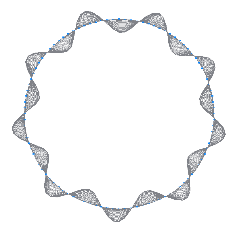
n = 0, 1, 2, ... - number of pairs of nodal lines in the meridian direction when each pair is located on one diameter.
The deviations from the theory for the initial natural frequencies are due to the fact that the natural modes and frequencies are determined by the program for a design model with all degrees of freedom of nodal displacements, i.e. tangential inertia forces were taken into account as well. These forces are especially noticeable in natural modes with a small number of half waves m in the circumferential direction.
The exact solution from the source does not take into account the tangential inertia forces. However, the page 440 of this handbook provides a formula for the estimation of the error introduced by this assumption. It gives a value of the correction to the square of the natural frequency:
k=1/(1+z).
For the first modes when m=2 the calculations gave the value z=0,042. Therefore, we can expect a 2% correction to the theoretical value.