Stability of a Rectangular Simply Supported Plate under Pure Shear

Objective: Determination of the critical value of the shear forces uniformly distributed along two opposite sides of a simply supported rectangular plate corresponding to the moment of its buckling.
Initial data files:
|
File name |
Description |
|---|---|
|
Design model with the ratios of the sides of the plate a/b = 1.0 5 from four-node shell elements of type 44 |
|
|
Design model with the ratios of the sides of the plate a/b = 1.0 from eight- node shell elements of type 50 |
|
|
Design model with the ratios of the sides of the plate a/b = 2.0 5 from four-node shell elements of type 44 |
|
|
Design model with the ratios of the sides of the plate a/b = 2.0 from eight- node shell elements of type 50 |
Problem formulation: The simply supported rectangular plate is subjected to the action of shear forces τ, uniformly distributed along two opposite sides. Determine the critical value of the shear forces τcr, corresponding to the moment of buckling of the rectangular plate.
References: S. P. Timoshenko, Stability of Bars, Plates and Shells, Moscow, Nauka, 1971, p. 626.
A.S. Volmir. Stability of Deformable Systems, Moscow, Nauka, 1967, p. 344.
Initial data:
| a = 8.0; 16.0 m | - side of the rectangular plate along the X axis of the global coordinate system; |
| b = 8.0 m | - side of the rectangular plate along the Y axis of the global coordinate system; |
| h = 0.08 m | - thickness of the rectangular plate; |
| E = 1.0·107 kN/m2 | - elastic modulus of the rectangular plate material; |
| ν = 1/3 | - Poisson’s ratio; |
| σ = 1.25·103 kN/m2 | - initial value of the shear forces. |
Finite element model: Design model – general type system. Two design models with four-node shell elements of type 44 and eight-node shell elements of type 50 are considered for two cases with the ratios of the sides of the plate a/b = 1.0; 2.0. The spacing of the finite element mesh along the sides of the plate (along the X and Y axes of the global coordinate system) is 1.0 m. Number of elements in the models – 64; 128. Boundary conditions are provided by imposing constraints on the nodes of the support contour of the plate in the direction of the degree of freedom Z. A load uniformly distributed along the line with the initial value p = -τ∙h = -100 kN/m is specified on one of the two opposite sides of the plate parallel to the X axis of the global coordinate system, and the constraints in the directions of the degrees of freedom X and Y are imposed on the nodes of the other one (lying on the X axis). A load uniformly distributed along the line with the initial value p = -τ∙h = -100 kN/m is specified on one of the two opposite sides of the plate parallel to the Y axis of the global coordinate system, and a load uniformly distributed along the line with the initial value p = τ∙h = 100 kN/m is specified on the other one (lying on the Y axis). The dimensional stability of the design model is provided by imposing a constraint in the UZ direction of the global coordinate system on the node of one of the corners of the plate. Number of nodes in the models – 81 (225); 153 (433).
Results in SCAD
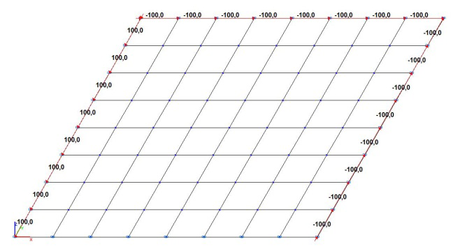
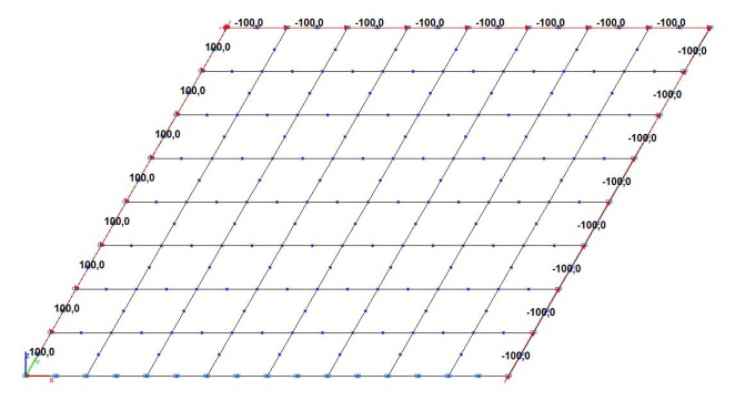
Design models with the ratio of the sides of the plate a/b = 1.0
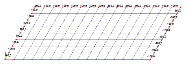
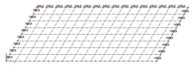
Design models with the ratio of the sides of the plate a/b = 2.0

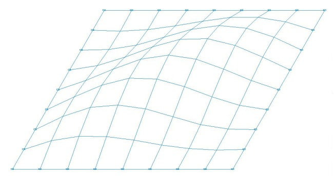
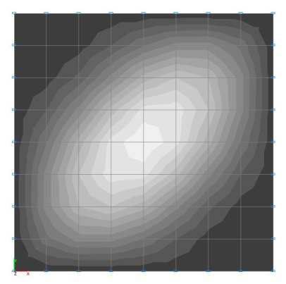
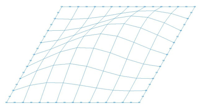
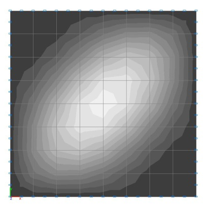
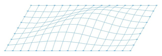
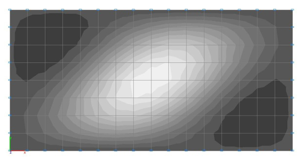
Buckling modes for the design models with the ratio of the sides of the plate a/b = 1.0
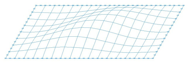
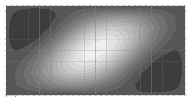
Buckling modes for the design models with the ratio of the sides of the plate a/b = 2.0
Comparison of solutions:
Critical value of the shear forces τcr, kN/m2
|
Plate sides ratio |
Design model |
Theory |
SCAD |
Deviation, % |
|---|---|---|---|---|
|
a/b = 1.0 |
Member type 44 n = 4 nodes |
8631 |
7.129409∙100/0.08 = = 8912 |
3.26 |
|
Member type 50 n = 8 nodes |
6.903095∙100/0.08 = = 8629 |
0.02 |
||
|
a/b = 2.0 |
Member type 44 n = 4 nodes |
6060 |
4.930113∙100/0.08 = = 6163 |
1.70 |
|
Member type 50 n = 8 nodes |
4.845765∙100/0.08 = = 6057 |
0.05 |
Notes: In the analytical solution the critical value of the shear forces τcr, corresponding to the moment of buckling of the rectangular plate can be determined according to the following formula:
\[ \sigma_{cr} =k\cdot \frac{\pi^{2}\cdot D}{b^{2}\cdot h}, \quad where: \quad \] \[ D=\frac{E\cdot h^{3}}{12\cdot \left( {1-\nu^{2}} \right)}, \quad k=\frac{\pi^{2}}{32\cdot \alpha^{3}\cdot \lambda }, \quad \alpha =\frac{a}{b}. \]
Parameter λ is determined on the basis of the condition of equality to zero of the determinant of the system of equations:
\[ \lambda \cdot \left( {m^{2}+\alpha^{2}\cdot n^{2}} \right)\cdot A_{mn} -\sum\limits_i {\sum\limits_j {\frac{m\cdot n\cdot i\cdot j}{\left( {m^{2}-i^{2}} \right)\cdot \left( {n^{2}-j^{2}} \right)}\cdot A_{ij} =0,} } \]
with the following combinations of indices:
| m + i n + j m + n |
odd odd even. |
At m, n, i, j = 1, 2, 3, 4, 5, 6, 7, 8 (the determinant dimension is 32∙32) we have:
\[ {\begin{array}{*{20}c} {\frac{a}{b}=1.0} & {k=9.328} \\ {\frac{a}{b}=2.0} & {k=6.549.} \\ \end{array} } \]