Double-Guyed Mast Subjected to Static Loads and Prestressing Forces

Objective: Determination of the stress state of a double-guyed mast subjected to static loads and prestressing forces in the physically nonlinear formulation.

Initial data file: Mast.spr

Problem formulation: The double-guyed mast with a trunk clamped in the support and cable stays symmetrically descending from its top at an angle α to the horizon is subjected to the following actions (in the plane of the mast structure):

• In the initial state the cable stays are subjected to the uniformly distributed shear load q_lg0 = q_rg0 and are prestressed with the force H₀;
• In the operating state the mast trunk is subjected to the uniformly distributed load q_m and to the moment Mm applied at its top, the windward and leeward cable stays are subjected to the uniformly distributed loads q_lg and q_rg, the temperature of the system does not change.

Determine the longitudinal forces N_lg, N_rg and N_m in the windward and leeward cable stays and in the mast trunk, as well as the bending moments M_m in the cross-sections of the mast trunk.

References: A. V. Perelmuter, Principles of Analysis of Cable-Bar Systems, Stroyizdat, 1969, p. 61

Initial data:

EFg = 0.58·105 t	- axial stiffness of the cable stays;
EIm = 0.92·107 t∙m2	- bending stiffness of the mast trunk;
S = 93.0 m	- height of the mast trunk;
L = 115.5 m	- length of the chord of the cable stays;
α = 45°	- angle of the cable stays to the horizon;
qlg0 = qrg0 = 22.75∙10-3∙cos(α) =16.087 t/m	- uniformly distributed shear load on the cable stays in the initial state;
qlg = 37.40∙10-3 - qlg0/ cos(α) = 14.650 t/m	- uniformly distributed shear load on the windward cable stay in the operating state;
qrg = qrg0/ cos(α) - 8.10∙10-3 = 14.650 t/m	- uniformly distributed shear load on the leeward cable stay in the operating state;
qm = 950.00∙10-3 t/m	- uniformly distributed shear load on the mast trunk in the operating state;
Mm = 401.00 t∙m	- moment at the top of the mast trunk;
H0 = 19.40 t	- prestressing forces of the cable stays.

 

Finite element model: Design model – general type system. Elements of the mast trunk – 93 bar elements of type 5. The spacing of the finite element mesh along the height of the mast trunk (along the X₁ axes of the local coordinate systems) is 1.0 m. Stiffness properties of the elements of the mast trunk:

EF = 1.00·10⁸ т;          EI_y = EI_z = GI_x = 0.92·10⁷ т·м².

Elements of the cable stays – 2 cable-stayed elements of type 308. Boundary conditions are provided by imposing constraints on the support nodes of the cable stays in the directions of the degrees of freedom X, Z and on the support node of the mast trunk in the directions of the degrees of freedom X, Z, UY.

Actions in the initial state are defined by the stiffness properties of the cable-stayed elements:

γ =  7.84483 t/m3	- specific weight of the cable stays;
E = 2.00·107 t/m2	- elastic modulus of the material of the cable stays;
ν = 0.3	- Poisson’s ratio;
H0 = 19.40 t	- prestressing forces of the cable stays;
D = 6.0675 cm	- outer diameter of the ring cross-section of the cable stays;
d = 0.0001 cm	- inner diameter of the ring cross-section of the cable stays.

 

A separate loading with a vertical concentrated load of the minimum value P₀ = 1.00∙10^-4  t applied at the top of the mast trunk is created to control the values of the internal forces in the initial state.

 

The actions in the operating state are specified as the following loads:

• uniformly distributed shear load in the local coordinate system along the Z₁ axis applied to the cable-stayed elements;
• uniformly distributed shear load in the global coordinate system along the X axis applied to the elements of the mast trunk;
• concentrated moment about the Y axis of the global coordinate system applied to the top node of the mast trunk.

The nonlinear loading was generated for the simple incremental method with a loading factor – 0.1 and a number of steps – 10 for the actions of the initial state, with a loading factor – 0.01 and a number of steps – 100 for the actions of the operating state.

Number of nodes in the design model – 96.

 

Results in SCAD

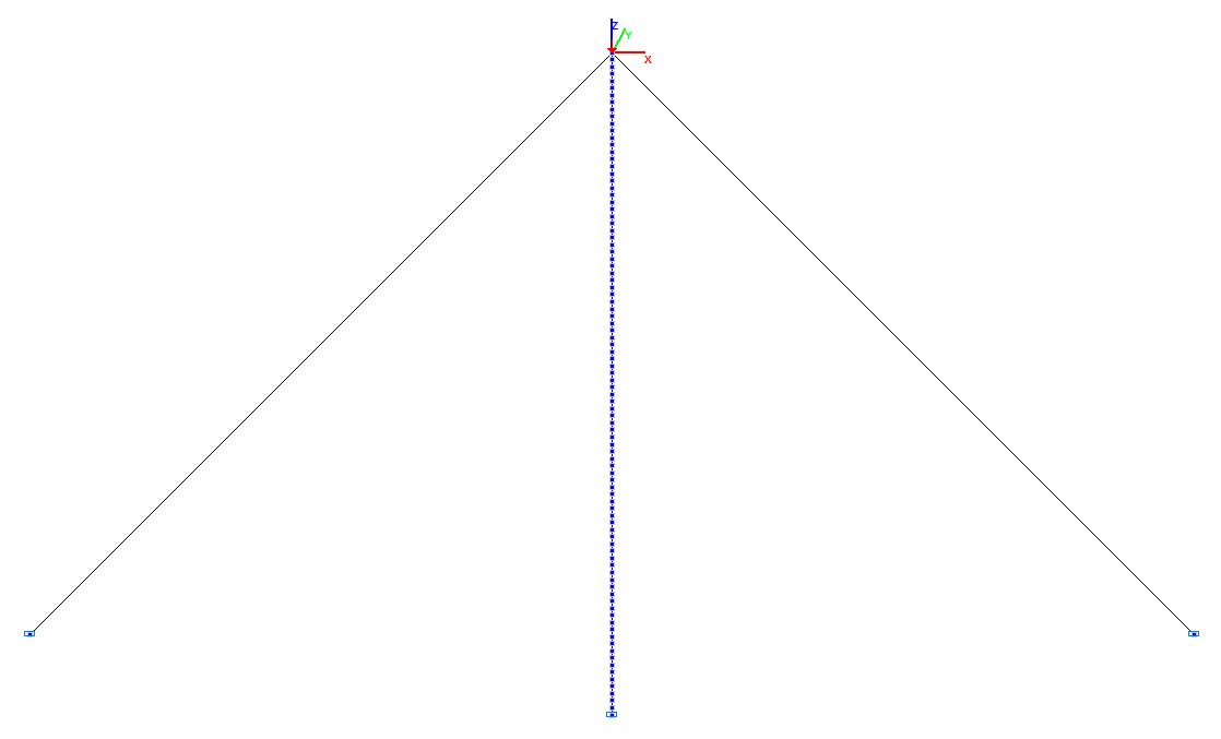
Design model in the initial state

 

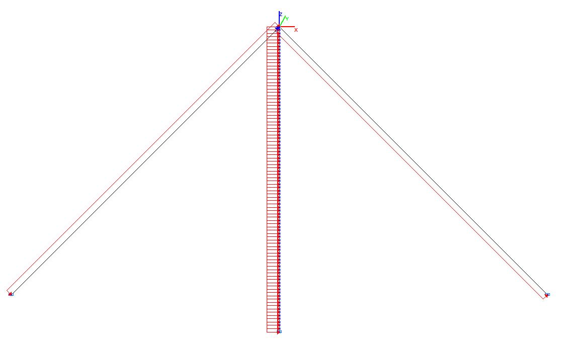
Design model in the operating state

 

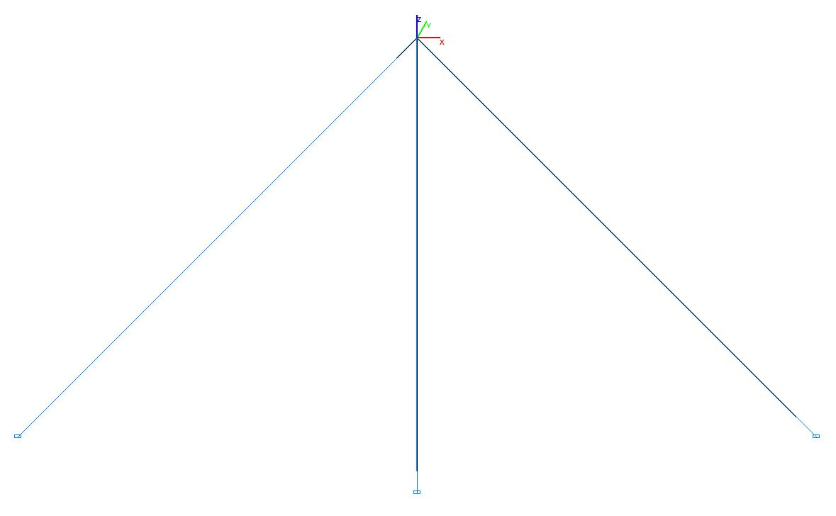
Deformed model in the initial state

 

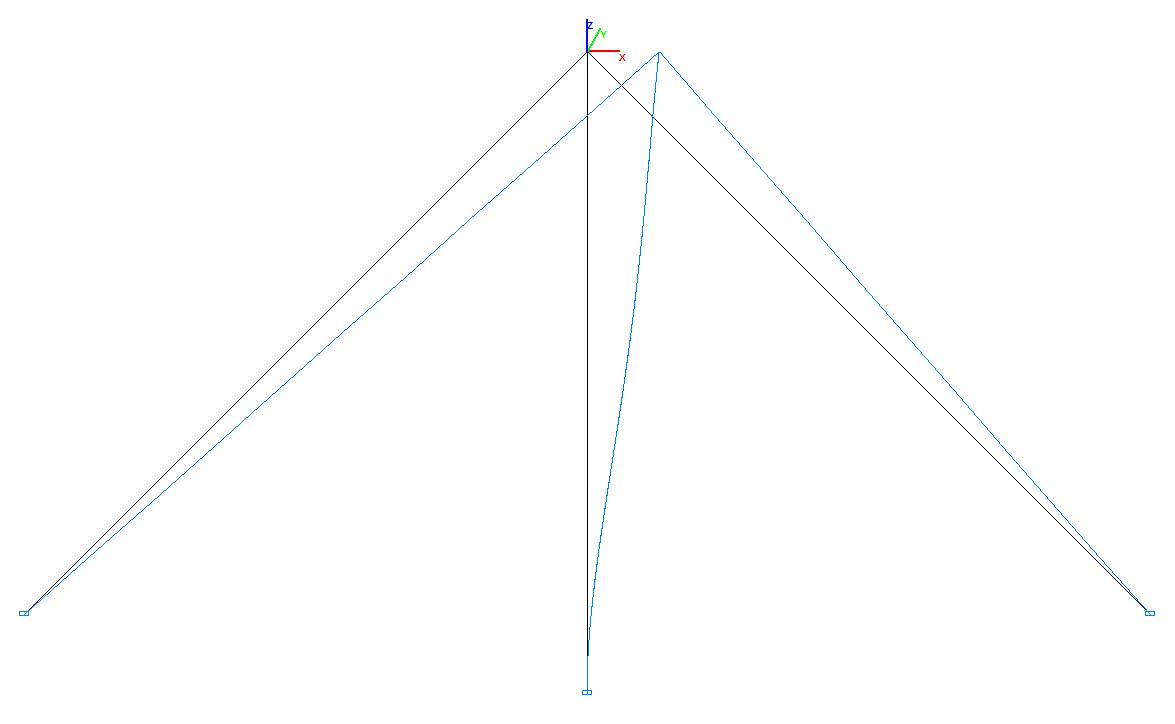
Deformed model in the operating state

 

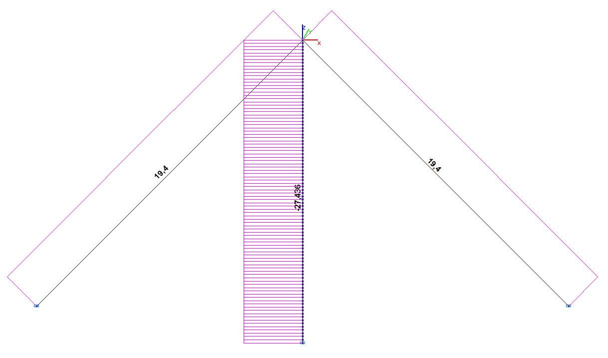
Longitudinal force diagrams in the initial state (т)

 

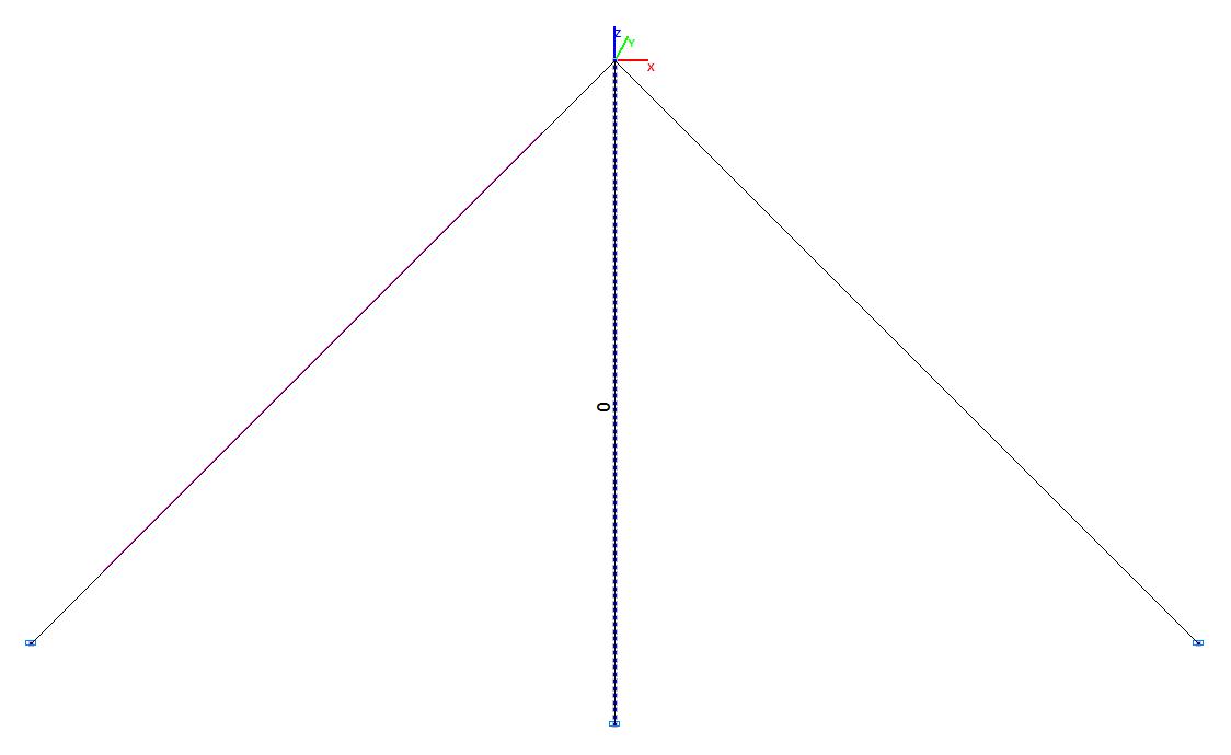
Bending moment diagrams in the initial state (t∙m)

 

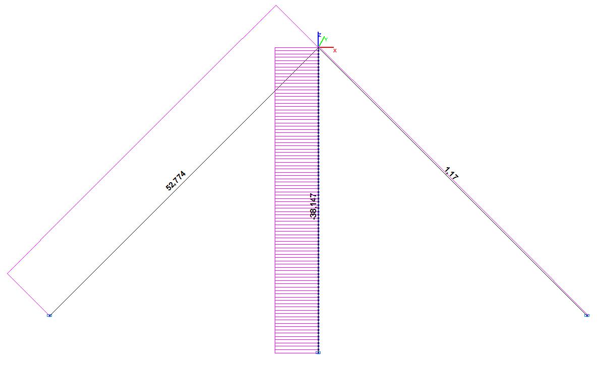
Longitudinal force diagrams in the operating state (t)

 

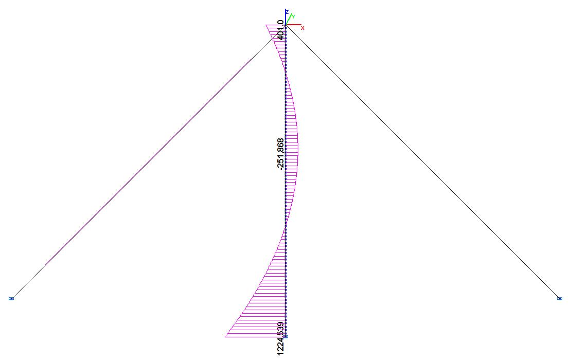
Bending moment diagrams in the operating state (t∙m)

 

Comparison of solutions:

Parameter	Theory	SCAD	Deviation, %
Nlg, t	52.769	52.774	0.01
Nrg, t	1.171	1.170	0.09
Nm, t	-38.142	-38.147	0.01
Mm(0), t∙m	1227.376	1224.539	0.23
Mm(S), t∙m	401.000	401.000	0.00
Sextr, m	55.853	56.000	―
Mm(Sextr), t∙m	-254.437	-251.868	1.01

Notes: In the analytical solution the internal forces in the twice statically indeterminate mast structure are determined by the force method, and the thrust reactions X₁ and X₂ of the support nodes of the cable stays are taken as the unknowns.

The values of the unknowns X₁ and X₂ are determined by solving the system of linear equations:

\[ {\begin{array}{*{20}c} {N_{\lg } =H_{0} +N_{\lg 1} \cdot X_{1} +N_{\lg q} ;} \\ {N_{rg} =H_{0} +N_{rg2} \cdot X_{2} +N_{rgq} ;} \\ {N_{m} =-2\cdot H_{0} \cdot \sin \left( \alpha \right)+N_{m1} \cdot X_{1} +N_{m2} \cdot X_{2} +N_{mq} ;} \\ {M_{m} \left( 0 \right)=M_{m1} \left( 0 \right)\cdot X_{1} +M_{m2} \left( 0 \right)\cdot X_{2} +M_{mq} \left( 0 \right);} \\ {M_{m} \left( S \right)=M_{m1} \left( S \right)\cdot X_{1} +M_{m2} \left( S \right)\cdot X_{2} +M_{mq} \left( S \right);} \\ {S_{extr} =S+\frac{q_{\lg } +q_{rg} }{q_{m} }\cdot L\cdot \sin \left( \alpha \right)+\frac{X_{1} -X_{2} }{q_{m} };} \\ {M_{m} \left( {S_{extr} } \right)=\frac{q_{m} }{2}\cdot S_{extr} ^{2}-\left[ {q_{m} \cdot S+\left( {q_{\lg } +q_{rg} } \right)\cdot L\cdot \sin \left( \alpha \right)+X_{1} -X_{2} } \right]\cdot S_{extr} +} \\ {\frac{q_{m} }{2}\cdot S^{2}+\left( {q_{\lg } +q_{rg} } \right)\cdot S\cdot L\cdot \sin \left( \alpha \right)+M_{m} +\left( {X_{1} -X_{2} } \right)\cdot S.} \\ \end{array} } \]

Значения неизвестных X₁ и X₂ определяются из решения системы линейных уравнений:

\[ \left. {{\begin{array}{*{20}c} {\left( {\frac{N_{\lg 1}^{2}\cdot L}{EF_{g} }+\frac{M_{m1}^{2}\left( 0 \right)\cdot S}{3\cdot EI_{m} }} \right)\cdot X_{1} +\frac{M_{m1} \left( 0 \right)\cdot M_{m2} \left( 0 \right)\cdot S}{3\cdot EI_{m} }\cdot X_{2} +\frac{N_{\lg 1} \cdot N_{\lg q} \cdot L}{EF_{g} }+} \\ {\frac{S}{6\cdot EI_{m} }\cdot \left( {M_{m1} \left( 0 \right)\cdot M_{mq} \left( 0 \right)+4\cdot M_{m1} \left( {\frac{S}{2}} \right)\cdot M_{mq} \left( {\frac{S}{2}} \right)+M_{m1} \left( S \right)\cdot M_{mq} \left( S \right)} \right)-} \\ {\frac{1}{2}\cdot N_{\lg 1} \cdot \left( {\frac{\left( {q_{\lg } +q_{\lg 0} } \right)^{2}\cdot L^{3}}{12\cdot \left( {H_{0} +N_{\lg q} +N_{\lg 1} \cdot X_{1} } \right)^{2}}-\frac{q_{\lg 0}^{2}\cdot L^{3}}{12\cdot H_{0}^{2}}} \right)=0} \\ {\frac{M_{m1} \left( 0 \right)\cdot M_{m2} \left( 0 \right)\cdot S}{3\cdot EI_{m} }\cdot X_{1} +\left( {\frac{N_{rg2}^{2}\cdot L}{EF_{g} }+\frac{M_{m2}^{2}\left( 0 \right)\cdot S}{3\cdot EI_{m} }} \right)\cdot X_{2} +\frac{N_{rg1} \cdot N_{rgq} \cdot L}{EF_{g} }+} \\ {\frac{S}{6\cdot EI_{m} }\cdot \left( {M_{m2} \left( 0 \right)\cdot M_{mq} \left( 0 \right)+4\cdot M_{m2} \left( {\frac{S}{2}} \right)\cdot M_{mq} \left( {\frac{S}{2}} \right)+M_{m2} \left( S \right)\cdot M_{mq} \left( S \right)} \right)-} \\ {\frac{1}{2}\cdot N_{rg2} \cdot \left( {\frac{\left( {-q_{rg} +q_{rg0} } \right)^{2}\cdot L^{3}}{12\cdot \left( {H_{0} +N_{rgq} +N_{rg2} \cdot X_{2} } \right)^{2}}-\frac{q_{rg0}^{2}\cdot L^{3}}{12\cdot H_{0}^{2}}} \right)=0} \\ \end{array} }} \right\}, \] \[ where: \quad N_{\lg 1} =-\frac{1}{\cos \left( \alpha \right)}; \quad N_{m1} =tg\left( \alpha \right); \] \[ M_{m1} \left( 0 \right)=1\cdot S; \quad M_{m1} \left( {\frac{S}{2}} \right)=\frac{S}{2}; \quad M_{m1} \left( S \right)=0\cdot S; \] \[ N_{rg2} =-\frac{1}{\cos \left( \alpha \right)}; \quad N_{m2} =tg\left( \alpha \right); \] \[ M_{m2} \left( 0 \right)=-1\cdot S; \quad M_{m2} \left( {\frac{S}{2}} \right)=-\frac{S}{2}; \quad M_{m2} \left( S \right)=-0\cdot S; \] \[ N_{\lg q} =-\frac{q_{\lg } \cdot L}{2}\cdot tg\left( \alpha \right); \quad N_{rgq} =\frac{q_{rg} \cdot L}{2}\cdot tg\left( \alpha \right); \] \[ N_{mq} =-\frac{\left( {q_{\lg } -q_{rg} } \right)\cdot L}{2}\cdot \frac{\cos \left( {2\cdot \alpha } \right)}{\cos \left( \alpha \right)}; \] \[ M_{mq} \left( 0 \right)=M_{m} +\frac{q_{m} \cdot S^{2}}{2}+\left( {q_{\lg } +q_{rg} } \right)\cdot S\cdot L\cdot \sin \left( \alpha \right); \] \[ M_{mq} \left( {\frac{S}{2}} \right)=M_{m} +\frac{q_{m} \cdot S^{2}}{8}+\frac{\left( {q_{\lg } +q_{rg} } \right)\cdot S\cdot L}{2}\cdot \sin \left( \alpha \right); \] \[ M_{mq} \left( S \right)=M_{m} . \]