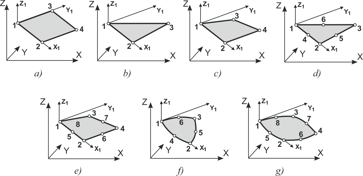
SCAD includes various flat finite elements with a triangular and quadrangular shape. The number of nodes in some types of elements can be greater than the number of vertices. In this case additional nodes lie on one or several sides of the element and their numbers follow after the numbers of vertices in any order.
These FEs are always located in the XOY plane and there are three degrees of freedom in each of their nodes: W — vertical displacement (deflection), and UX, UY — rotation angles about the X and Y axes. The FEs can be used in the models with indices 3, 5, 8 and 9 and have an isotropic, orthotropic, or anisotropic material. Moments MX, MY, MXY and shear forces QX and QY are calculated. When the subsoil parameter С1 is specified, RZ is calculated.
Figure 1. Plate finite elements
The list of FEs for the analysis of thin flexural plates is given in Table 1.
Table 1
Type |
Name |
Number of nodes |
Node numbering order and local axes |
Comments |
|---|---|---|---|---|
11 |
Rectangular |
4 |
Fig. 1, a |
semi-compatible [18, 22, 23] |
12, 14 |
Triangular |
3 |
Fig. 1, b |
incompatible [18, 22, 23] |
13 |
Rectangular |
4 |
Fig. 1, a |
incompatible [28] |
15 |
Triangular |
3-6 |
Fig. 1, d |
|
16 |
Quadrangular |
4-8 |
Fig. 1, e |
SubAreas, option 2 [25, 23] |
18 |
Triangular |
3-6 |
Fig. 1, d |
SubAreas, option 2 [24, 23] |
19 |
Quadrangular |
4 |
Fig. 1, c |
SubAreas, [25, 23] |
20 |
Quadrangular |
4-8 |
Fig. 1, e |
SubAreas, [24, 23], option 1 |
1 SubAreas – subdomain method: triangular and quadrangular elements are divided, respectively, by medians and diagonals into triangles. Approximation polynomials of the appropriate degree are used on each of these triangles in such a way that compatibility is ensured. We obtain piecewise polynomial approximations.
These elements are used for the analysis of medium thickness plates and implement the Reissner-Mindlin theory. They are completely similar to the elements used for the analysis of thin plates in terms of the specification of the initial data. They differ from the elements given in Table 1 only in their type number, which is greater by 100. For example, element 120 is a quadrangular element with the number of nodes from 4 to 8, similarly to the element 20.
Each node of the elements has three degrees of freedom: w — vertical displacement (deflection), the positive direction of which coincides with the direction of the Z axis, and the rotation angles UX and UY about the X and Y axes.
Table 2
Type |
Name |
Number of nodes |
Node numbering order and local axes |
Comments |
|---|---|---|---|---|
111 |
Rectangular |
4 |
Fig. 1, a |
|
112 |
Triangular |
3 |
Fig. 1, b |
JIDR3 [91, 23] |
115 |
Triangular |
3-6 |
Fig. 1, d |
JIDR3-6 [91, 23] |
116 |
Quadrangular |
4-8 |
Fig. 1, g |
isoparametric, JIDR [91, 23] |
118 |
Triangular |
3-6 |
Fig. 1, f |
isoparametric, JIDR [91, 23] |
119 |
Quadrangular |
4 |
Fig. 2, b |
JIDR [91, 23] |
120 |
Quadrangular |
4-8 |
Fig. 1, e |
JIDR, SubAreas [91, 23] |
512 |
Triangular |
3 |
Fig. 1, b |
|
517 |
Quadrangular |
4 |
Fig. 1, c |
|
518 |
Triangular |
3 |
Fig. 1, b |
DSG3 [76] |
The list of FEs for the analysis of plates according to the Reissner-Mindlin theory is given in Table 2.
2 JIDR, joint interpolation of displacements and rotations [91, 23].
3 DSG, Discrete Shear Gap [76].
4 MITC, Mixed Interpolation of Tensorial Components [3, 75].
All elements considered in this section enable to analyze both plane-stress and plane-strain systems (depending on the index, which is specified when describing the stiffness properties of the elements).
There are the following groups of element types:
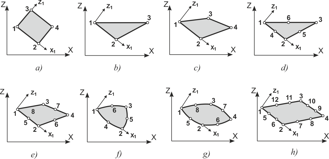
Figure 2. Plane finite elements
Table 3
Degrees of freedom of nodes |
Type |
Name |
Number of nodes |
Node numbering order and local axes |
Comments |
|---|---|---|---|---|---|
X, Z |
21 |
Rectangular |
4 |
Fig. 2, a |
polylinear shape functions |
22 |
Triangular |
3 |
Fig. 2, b |
linear shape functions |
|
25 |
Triangular |
3-6 |
Fig. 2, d |
SubAreas [16, 23] |
|
29 |
Quadrangular |
4-12 |
Fig. 2, h |
SubAreas [26, 23] |
|
30 |
Quadrangular |
4-8 |
Fig. 2, e |
SubAreas [26, 23] |
|
X, Y, Z |
23 |
Rectangular |
4 |
Fig. 2, a |
polylinear shape functions |
24 |
Triangular |
3 |
Fig. 2, b |
linear shape functions |
|
26 |
Quadrangular |
4-8 |
Fig. 2, g |
isoparametric |
|
27 |
Quadrangular |
4-8 |
Fig. 2, e |
SubAreas [26, 23] |
|
28 |
Triangular |
3-6 |
Fig. 2, f |
isoparametric |
|
Elements with drilling (DDF) and quasi-rotational degrees of freedom (QRDF) |
|||||
X, Y, UY |
121 |
Rectangular |
4 |
Fig. 2, a |
|
122 |
Triangular |
3 |
Fig. 2, b |
DDF, incompatible [90, 23] |
|
125 |
Triangular |
3-6 |
Fig. 2, d |
DDF, SubAreas [90, 23] |
|
129 |
Quadrangular |
4-8 |
Fig. 2, e |
DDF, SubAreas, incompatible [90, 23] |
|
130 |
Quadrangular |
4-8 |
Fig. 2, e |
DDF, SubAreas [90, 23] |
|
526 |
Quadrangular |
4 |
Fig. 2, c |
||
527 |
Quadrangular |
4 |
Fig. 2, c |
QRDF, SubAreas [90, 23] |
|
528 |
Triangular |
3 |
Fig. 2, b |
QRDF [90, 23] |
|
All elements can have isotropic, orthotropic or anisotropic material, as well as transverse isotropic for plane deformation.
The list of elements and their main properties are given in Table 3.
The following stresses are calculated — NX, NZ, NXZ, as well as NY — at the analysis of structures in the plane strain state. When the subsoil parameter Сuv is specified, Rx and Rz are calculated.
5 This can be either an average rotation angle or a quasi-rotational degree of freedom [90].
6 DDF – Drilling degrees of freedom[23]
7 QRDF – Quasi-rotational degrees of freedom [23]
Finite elements used for the analysis of thin shallow shells can take any position in space. Six degrees of freedom are determined in the nodes of the elements — U, V, W, UX, UY and UZ (three linear displacements along and three rotation angles about the coordinate axes). The degrees of freedom U, V correspond to the membrane deformations, and W, UX, UY correspond to the bending ones.
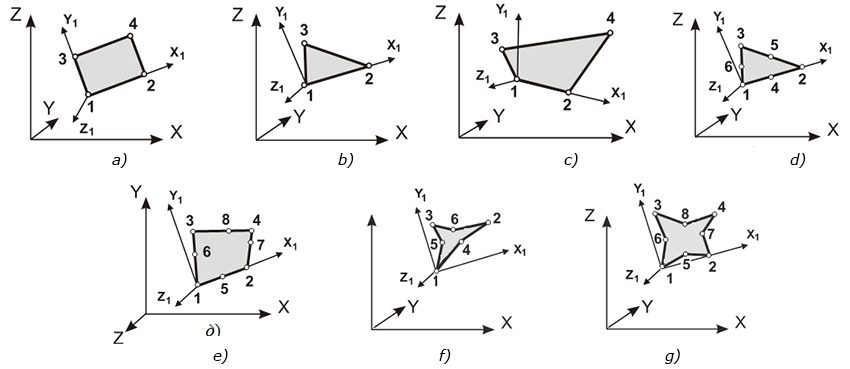
Figure 3. Shell elements
There are the following groups of element types:
Material — isotropic, orthotropic, and anisotropic.
The list of elements is given in Table 4.
Table 4
Type |
Name |
Number of nodes |
Node numbering order and local axes |
Degrees of freedom |
Comments |
|---|---|---|---|---|---|
41 |
Rectangular |
4 |
Fig. 3, a |
U, V |
polylinear shape functions |
W, UX, UY |
semi-compatible [18, 22, 23] |
||||
42 |
Triangular |
3 |
Fig. 3, b |
U, V |
linear shape functions |
W, UX, UY |
incompatible [18, 22, 23] |
||||
43 |
Rectangular |
4 |
Fig. 3, a |
U, V |
polylinear shape functions |
W, UX, UY |
incompatible [28, 23] |
||||
44 |
Quadrangular |
4 |
Fig. 3, c |
U, V |
SubAreas [26, 23] |
W, UX, UY |
SubAreas [25, 23] |
||||
45 |
Triangular |
3-6 |
Fig. 3, d |
U, V |
SubAreas [16, 23] |
W, UX, UY |
SubAreas [24, 23], option 1 |
||||
46 |
Quadrangular |
4-8 |
Fig. 3, c |
U, V |
SubAreas [26, 23] |
W, UX, UY |
SubAreas, option 2 [25, 23] |
||||
48 |
Triangular |
3-6 |
Fig. 3, d |
U, V |
SubAreas [16, 23] |
W, UX, UY |
SubAreas, option 2 [24, 23] |
||||
50 |
Quadrangular |
4-8 |
Fig. 3, e |
U, V |
SubAreas [26, 23] |
W, UX, UY |
SubAreas, option 1 [26, 23] |
||||
Elements with drilling (DDF) and quasi-rotational degrees of freedom (QRDF) |
|||||
91 |
Rectangular |
4 |
Fig. 3, a |
U, V, UZ |
DDF, incompatible [90, 23] |
W, UX, UY |
semi-compatible [18, 22, 23] |
||||
92 |
Triangular |
3 |
Fig. 3, b |
U, V, UZ |
DDF, incompatible [90, 23] |
W, UX, UY |
incompatible [18, 22, 23] |
||||
93 |
Rectangular |
4 |
Fig. 3, a |
U, V, UZ |
DDF, incompatible [90, 23] |
W, UX, UY |
incompatible [28, 23] |
||||
94 |
Quadrangular |
4 |
Fig. 3, e |
U, V, UZ |
DDF, SubAreas, incompatible [90, 23] |
W, UX, UY |
SubAreas, [25, 23] |
||||
95 |
Triangular |
3-6 |
Fig. 3, d |
U, V, UZ |
DDF, SubAreas [90, 23] |
W, UX, UY |
SubAreas [25, 23] |
||||
96 |
Quadrangular |
4-8 |
Fig. 3, e |
U, V, UZ |
DDF, SubAreas [90, 22] |
W, UX, UY |
SubAreas [25, 23] |
||||
97 |
Quadrangular |
4-8 |
Fig. 3, e |
U, V, UZ |
DDF, SubAreas, incompatible [90, 23] |
W, UX, UY |
SubAreas [25, 23] |
||||
591 |
Rectangular |
4 |
Fig. 3, a |
U, V, UZ |
QRDF4 [90, 23] |
W, UX, UY |
semi-compatible [18, 22, 23] |
||||
592 |
Triangular |
3 |
Fig. 3, b |
U, V, UZ |
QRDF3 [90, 23] |
W, UX, UY |
incompatible [18, 22, 23] |
||||
593 |
Rectangular |
4 |
Fig. 3, c |
U, V, UZ |
QRDF4, [90, 23] |
W, UX, UY |
incompatible [28, 23] |
||||
594 |
Quadrangular |
4 |
Fig. 3, c |
U, V, UZ |
QRDF4, SubAreas [23] |
W, UX, UY |
SubAreas [25, 23] |
||||
Stresses NX, NY, NXY, moments MX, MY, MXY and shear forces QX and QY are calculated. When the subsoil parameter СY specified, Rz is calculated, and when Сuv is specified, Rx and Ry are calculated.
The graphic postprocessor calculates also the forces in the plate section SNX, SNZZ, SNXZ.
These elements are used for the analysis of shallow shells allowing for shear and implement the Reissner-Mindlin theory. They are completely similar to the elements used for the analysis of thin shells in terms of the specification of the initial data.
The list of elements is given in Table 5.
Table 5
Type |
Name |
Number of nodes |
Node numbering order and local axes |
Degrees of freedom |
Comments |
|---|---|---|---|---|---|
141 |
Rectangular |
4 |
Fig. 3, а |
U, V |
polylinear shapes |
W, UX, UY |
JIDR, incompatible [91, 23] |
||||
142 |
Triangular |
3 |
Fig. 3, b |
U, V |
linear shape functions |
W, UX, UY |
JIDR3 [91, 23] |
||||
143 |
Quadrangular isoparametric |
4 |
Fig. 3, с |
U, V |
polylinear shape functions |
W, UX, UY |
MITC4, isoparametric [3, 75, 23] |
||||
144 |
Quadrangular |
4 |
Fig. 3, с |
U, V |
SubAreas [26, 23] |
W, UX, UY |
JIDR4, SubAreas [91, 23] |
||||
145 |
Triangular |
3-6 |
Fig. 3, d |
U, V |
SubAreas [26, 23] |
W, UX, UY |
JIDR, SubAreas [91, 23] |
||||
146 |
Quadrangular isoparametric |
4-8 |
Fig. 3, e |
U, V |
isoparametric |
W, UX, UY |
JIDR, isoparametric [91, 23] |
||||
147 |
Triangular, isoparametric |
3-6 |
Fig. 3, f |
U, V |
isoparametric |
W, UX, UY |
JIDR, isoparametric [91, 23] |
||||
148 |
Triangular
|
3 |
Fig. 3, b |
U, V |
linear shape functions |
W, UX, UY |
DSG3M [23] |
||||
149 |
Triangular
|
3 |
Fig. 3, b |
U, V |
linear shape functions |
W, UX, UY |
DSG3 [76, 23] |
||||
150 |
Quadrangular |
4-8 |
Fig. 3, e |
U, V |
JIDR, SubAreas [26, 23] |
W, UX, UY |
JIDR, SubAreas [91, 23] |
||||
Elements with drilling (DDF) and quasi-rotational degrees of freedom (QRDF) |
|||||
191 |
Rectangular |
4 |
Fig. 3, a |
U, V, UZ |
DDF, incompatible [90, 23] |
W, UX, UY |
JIDR [91, 23] |
||||
192 |
Triangular |
3 |
Fig. 3, b |
U, V, UZ |
DDF, SubAreas, [90, 23] |
W, UX, UY |
JIDR, SubAreas [91, 23] |
||||
194 |
Quadrangular |
4 |
Fig. 3, с |
U, V, UZ |
DDF, SubAreas [90, 23] |
W, UX, UY |
JIDR, SubAreas [91, 23] |
||||
195 |
Triangular |
3-6 |
Fig. 3, d |
U, V, UZ |
DDF, SubAreas [90, 23] |
W, UX, UY |
JIDR, SubAreas [91, 23] |
||||
196 |
Quadrangular |
4-8 |
Fig. 3, e |
U, V, UZ |
DDF, SubAreas [90, 23] |
W, UX, UY |
JIDR, SubAreas, [91, 23] |
||||
197 |
Quadrangular |
4-8 |
Fig. 3, e |
U, V, UZ |
DDF, incompatible, SubAreas [90, 23] |
W, UX, UY |
JIDR, SubAreas, [91, 2QRDF3] |
||||
542 |
Triangular |
3 |
Fig. 3, b |
U, V, UZ |
|
W, UX, UY |
JIDR [91, 23] |
||||
543 |
Quadrangular |
4 |
Fig. 3, с |
U, V, UZ |
QRDF, isoparametric [90, 23] |
W, UX, UY |
MITC4, isoparametric [3, 75, 23] |
||||
544 |
Quadrangular |
4 |
Fig. 3, а |
U, V, UZ |
QRDF, SubAreas [90, 23] |
W, UX, UY |
JIDR, SubAreas [91, 23] |
||||
546 |
Quadrangular |
4 |
Fig. 3, с |
U, V, UZ |
QRDF, isoparametric [90, 23] |
W, UX, UY |
JIDR, isoparametric [91, 23] |
||||
547 |
Triangular |
4 |
Fig. 3, b |
U, V, UZ |
QRDF [90, 23] |
W, UX, UY |
DSG3M [23] |
||||
548 |
Triangular |
3 |
Fig. 3, b |
U, V, UZ |
QRDF [90, 23] |
W, UX, UY |
DSG3 [76, 23] |
||||